Electrochemistry Class 12 Notes: CBSE Chemistry Chapter 2

Electrochemistry

Electrochemistry is the study of generating electricity from the energy produced during a spontaneous chemical reaction, as well as the application of electrical energy to non-spontaneous chemical changes.

Electrochemical Cells

A spontaneous chemical reaction is one that can occur on its own, and in such a reaction, the system's Gibbs energy falls. This energy is then transformed into electrical energy. It is also feasible to force non-spontaneous processes to occur by providing external energy in the form of electrical energy. Electrochemical Cells are used to carry out these interconversions. 

Types

Two types of electrochemical cells are present: Galvanic cells, which converts chemical energy into electrical energy and electrolytic cells which converts electrical energy into chemical energy.

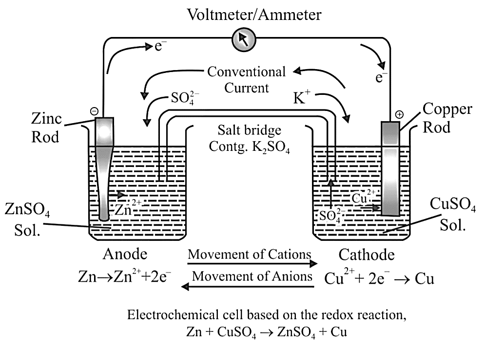
Galvanic Cells

A spontaneous chemical process or reaction is used to extract cell energy, which is then transformed to electric current.

For example, a Daniell Cell is a Galvanic Cell in which the redox reaction is carried out using Zinc and Copper.

$Zn(s) + C{u^{2 + }}(aq) \to Z{n^{2 + }}(aq) + Cu(s)$ 

Oxidation Half: $Zn(s) \to Z{n^{2 + }}(aq) + 2{e^ - }$ 

Reduction Half: $C{u^{2 + }}(aq) + 2{e^ - } \to Cu(s)$ 

The reducing agent is $Zn$ , and the oxidising agent is $C{u^{2 + }}$ .

Electrodes are another name for half cells. The anode is the oxidation half, and Cathode is the reduction half. The cathode is a term used to describe a type of electrode. In the external circuit, electrons pass from the anode to the cathode. Negative polarity is assigned to the anode. Positive polarity is assigned to the cathode. Daniell Cell is a fictional character created by Daniell Cell. The anode is $Zn$ , while the cathode is $Cu$ .

Electrolytic Cell

These electrodes are submerged in an electrolytic solution that contains both cations and anions. When current is supplied, the ions migrate towards electrodes of opposite polarity, where they undergo simultaneous reduction and oxidation.

Preferential Discharge of Ions

When more than one cation or anion is present, the discharge process becomes competitive. Any ion that needs to be discharged requires energy, and if there are multiple ions present, the ion that requires the most energy will be discharged first.

Electrode Potential

It can be defined as an element's tendency to lose or gain electrons when in contact with its own ions, causing it to become positively or negatively charged. Depending on whether oxidation or reduction has occurred, the electrode potential will be referred to as oxidation or reduction potential.

$M(s)\underset{{{\text{Reduction}}}}{\overset{{{\text{Oxidation}}}}{\longleftrightarrow}}{M^{n + }}(aq) + n{e^ - }$

${M^{n + }}(aq) + n{e^ - }\underset{{{\text{Oxidation}}}}{\overset{{{\text{Reduction}}}}{\longleftrightarrow}}M(s)$

Characteristics

1. The magnitude and sign of the oxidation and reduction potentials are equal. 

2. Because E is not a thermodynamic property, its values do not add up.

Standard Electrode Potential $({E^ \circ })$ 

It can be described as an electrode's electrode potential measured in comparison to a standard hydrogen electrode under standard conditions. The following are the standard conditions:

1. A 1M concentration of each ion in the solution.

2. A 298 K temperature.

3. Each gas has a pressure of one bar.

Electrochemical Series

The half-cell potential values are standard and are represented as standard reduction potential values in the table at the conclusion, commonly known as the Electrochemical Series.

Cell Potential or EMF of a Cell

Cell potential is the difference between the electrode potentials of two half-cells. If no current is pulled from the cell, it is known as electromotive force (EMF). 

${E_{cell}} = {E_{cathode}} + {E_{anode}}$ 

For this equation, we take the oxidation potential of the anode and the reduction potential of the cathode. 

Since the anode is put on the left and the cathode on the right, it follows therefore:

$ = {E_R} + {E_L}$ 

For a Daniel Cell, therefore:

$E_{cell}^ \circ  = E_{C{u^{2 + }}/Cu}^ \circ  - E_{Zn/Z{n^{2 + }}}^ \circ  = 0.34 + (0.76) = 1.10\;V$

Cell Diagram or Representation of a Cell

In accordance with IUPAC recommendations, the following conventions or notations are used to write the cell diagram. The Daniel cell has the following representation:

$Zn(s)|Z{n^{2 + }}({C_1})||C{u^{2 + }}({C_2})|Cu(s)$ 

1. The anode half cell is written on the left, while the cathode half cell is written on the right. 

2. The metal is separated from an aqueous solution of its own ions by a single vertical line.

Anodic Chamber: $Zn(s)|Z{n^{2 + }}(aq)$ 

Cathodic Chamber: $C{u^{2 + }}(aq)|Cu(s)$ 

3. A salt bridge is represented by a double vertical line.

4. After the formula of the corresponding ion, the molar concentration (C) is placed in brackets.

5. The cell's e.m.f. value is written on the cell's extreme right side. As an example:

$Zn(s)|Z{n^{2 + }}(1M)||C{u^{2 + }}(1M)|Cu$ , EMF = +1.1 V

6. If an inert electrode, such as platinum, is used in the cell's construction, it may be written in brackets alongside the working electrode, as when a zinc anode is coupled to a hydrogen electrode. 

$Zn(s)|Z{n^{2 + }}({C_1})||{H^ + }({C_2})|{H_2}(Pt)(s)$ 

Salt Bridge

The salt bridge maintains charge balance and completes the circuit by allowing ions to flow freely through it. It contains a gel containing an inert electrolyte such as $N{a_2}S{O_4}$  or $KN{O_3}$ . Through the salt bridge, negative ions travel to the anode and positive ions flow to the cathode, maintaining charge balance and allowing the cell to function.

Spontaneity of a Reaction

$\Delta G =  - nF{E_{cell}}$ 

$\Delta G$ should be negative and cell potential should be positive for a spontaneous cell reaction.

In the following equation, if we take the standard value of cell potential, we will also get the standard value of $\Delta G$ .

$\Delta {G^ \circ } =  - nFE_{CELL}^ \circ $ 

Types of Electrodes

Metal – Metal Ion Electrodes

An electrolyte solution containing metal ions is dipped into a metal rod/plate. Because of the potential difference between these two phases, this electrode can function as both a cathode and an anode.

Anode: $M \to {M^{n + }} + n{e^ - }$ 

Cathode: ${M^{n + }} + n{e^ - } \to M$ 

Gas Electrodes

Electrode gases such as ${H_2}$  and $C{l_2}$  are used in conjunction with their respective ions. ${H_2}$  gas, for example, is utilised in conjunction with a dilute solution of $HCl$  (${H^ + }$  ions). To avoid reacting with the acid, the metal should be inert. 

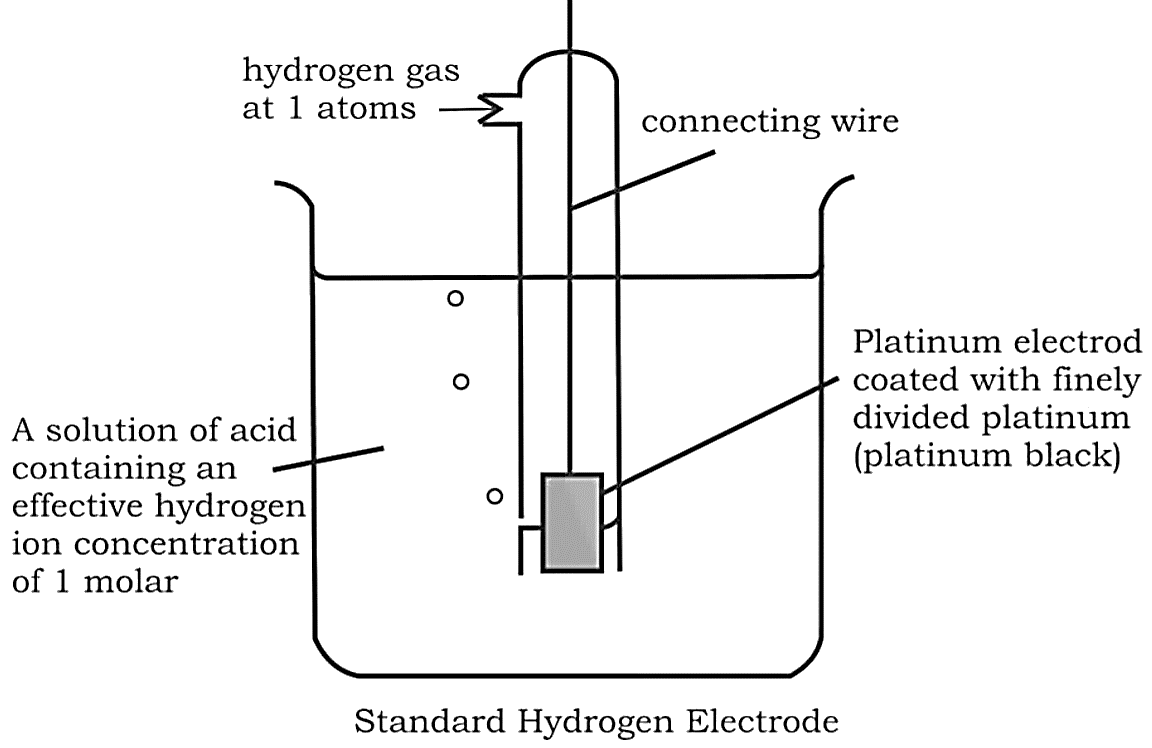
Anode: ${H_2} \to 2{H^ + } + 2{e^ - }$

Cathode: $2{H^ + } + 2{e^ - } \to {H_2}$ 

The hydrogen electrode is also used as a standard for measuring the potentials of other electrodes. As a reference, its own potential is set at $0\;V$ . The concentration of the HCl used as a reference is 1 M, and the electrode is known as the "Standard Hydrogen Electrode (SHE)".

Metal – Insoluble Salt Electrode

As electrodes, we use salts of several metals that are only sparingly soluble with the metal itself. When we employ $AgCl$  with $Ag$ , for example, there is a potential gap between these two phases, as seen in the following reaction:

$AgCl(s) + {e^ - } \to Ag(s) + C{l^ - }$ 

This electrode is made by dipping a silver rod in a solution containing $AgCl(s)$  and $C{l^ - }$  ions.

Calomel Electrode

Mercury is combined with two other phases: calomel paste $(H{g_2}C{l_2})$  and a $C{l^ - }$ ions containing electrolyte.

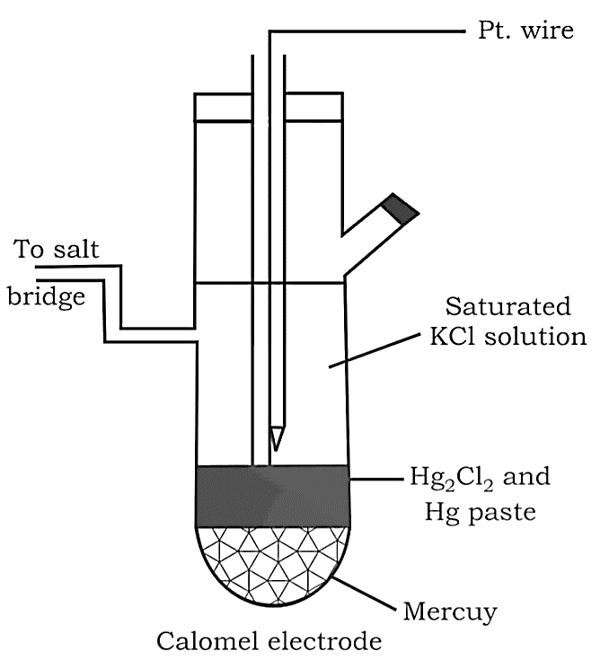
Cathode: $H{g_2}C{l_2}(s) + 2{e^ - } \to 2Hg(l) + 2C{l^ - }(aq)$ 

Anode: $2Hg(l) + 2C{l^ - }(aq) \to H{g_2}C{l_2}(s) + 2{e^ - }$ 

This electrode is also utilised as a reference point for determining other potentials. It's also known as Standard Calomel Electrode in its standard form (SCE).

Redox Electrode

Two distinct oxidation states of the same metal are used in the same half cell in these electrodes. For example, $F{e^{2 + }}$  and $F{e^{3 + }}$  are dissolved in the same container and the electron transfer is performed using a platinum inert electrode.

The following reactions may occur:

Anode: $F{e^{2 + }} \to F{e^{3 + }} + {e^ - }$

Cathode: $F{e^{3 + }} + {e^ - } \to F{e^{2 + }}$ 

Nernst Equation

It establishes a link between electrode voltage and ion concentration. When a result, as the concentration of ions rises, so does the reduction potential. For a type of generic electrochemical reaction.

$aA + bB\xrightarrow{{n{e^ - }}}cC + dD$ 

Nernst equation can be given as:

${E_{{\text{cell}}}} = E_{{\text{call}}}^0 - \dfrac{{RT}}{{nF}}\ln \dfrac{{{{[C]}^c}{{[D]}^d}}}{{{{[A]}^a}{{[B]}^b}}}$

 ${E_{c \in l}} = E_{cdl}^ \circ  - \dfrac{{2303}}{{nF}}RT\log \dfrac{{{{[C]}^c}{{[D]}^d}}}{{{{[A]}^a}{{[B]}^b}}}$

Substituting the values of R and F we get:

 ${E_{{\text{cell}}}} = E_{ccll}^0 - \dfrac{{0.0591}}{n}\log \dfrac{{{{[C]}^c}{{[D]}^d}}}{{{{[A]}^a}{{[B]}^b}}}$

Applications of Nernst Equation

Equilibrium Constant from Nernst Equation

For a Daniel Cell, at equilibrium

${{E_{{\text{cell}}}} = 0 = E_{{\text{cell}}}^0 - \dfrac{{2.303{\text{RT}}}}{{2{\text{F}}}}\log \dfrac{{\left[ {{\text{Z}}{{\text{n}}^{2 + }}} \right]}}{{\left[ {{\text{C}}{{\text{u}}^{2 + }}} \right]}}}$

${{\text{E}}_{{\text{cdl}}}^{\text{o}} = \dfrac{{2.303{\text{RT}}}}{{2{\text{F}}}}\log \dfrac{{\left[ {{\text{Z}}{{\text{n}}^{2 + }}} \right]}}{{\left[ {{\text{C}}{{\text{u}}^{2 + }}} \right]}}}$ 

But at equilibrium:

 $\dfrac{{\left[ {Z{n^{2 + }}} \right]}}{{\left[ {C{u^{2 + }}} \right]}} = {K_c}$

${{\text{E}}_{cell}^{\text{a}} = \dfrac{{2.303{\text{RT}}}}{{2{\text{F}}}}\log {{\text{K}}_{\text{c}}}}$

${{\text{E}}_{cell}^{\text{o}} = \dfrac{{2.303 \times 8.314 \times 298}}{{2 \times 96500}}\log {{\text{K}}_{\text{c}}}}$

  ${ = \dfrac{{0.0591}}{2}\log {{\text{K}}_{\text{c}}}}$ 

In general:

${{\text{E}}_{{\text{cell}}}^ \circ  = \dfrac{{0.0591}}{{\text{n}}}\log {{\text{K}}_{\text{c}}}}$ 

${\log {{\text{K}}_{\text{c}}} = \dfrac{{{\text{n}}E_{{\text{cell}}}^ \circ }}{{0.0591}}}$

Concentration Cells

Concentration cells are formed when two electrodes of the same metal are dipped individually into two solutions of the same electrolyte with varying concentrations and the solutions are connected by a salt bridge. As an example:

${H_2}|{H^ + }({C_1})||{H^ + }({C_2})|{H_2}$ 

$Cu|C{u^{ + 2}}({C_1})||C{u^{2 + }}({C_2})|Cu$ 

These Are of Two Types:

Electrode Concentration Cells

${H_2}({P_1})|{H^ + }(C)||{H^ + }(C)|{H_2}({P_2})$ 

${E_{{\text{cell}}}} = 0 - \dfrac{{0.059}}{n}\log \dfrac{{{P_2}}}{{{P_1}}}$

Where, ${P_2} < {P_1}$ for spontaneous reaction.

Electrolyte Concentration Cell

The EMF of concentration cell at 298 K is given by:

$Zn|Z{n^{2 + }}({C_1})||Z{n^{2 + }}({C_2})|Zn$ 

${{\text{E}}_{{\text{cell}}}} = \dfrac{{0.0591}}{{{{\text{n}}_1}}}\log \dfrac{{{{\text{c}}_2}}}{{{{\text{c}}_{\text{l}}}}}$

Where, ${C_2} > {C_1}$ for spontaneous reaction

Cases of Electrolysis

Electrolysis of Molten Sodium Chloride

$2NaCl(l) \rightleftharpoons 2N{a^ + }(l) + 2C{l^ - }(l)$

The reactions occurring at the two electrodes may be shown as follows:

At cathode: $2N{a^ + } + 2{e^ - } \to 2Na$ , ${E^ \circ } =  - 2.71\;V$

At anode: $2C{l^ - } \to C{l_2} + 2{e^ - }$ , ${E^ \circ } =  - 1.36\;V$ 

Overall reaction:

$2N{a^ + }(l) + 2C{l^ - }\xrightarrow{{electrolysis}}2Na(l) + C{l_2}(g)$ OR

$2NaCl(l)\xrightarrow{{electrolysis}}2Na(l) + C{l_2}(g)$ 

Electrolysis of an aqueous solution of Sodium Chloride

$NaCl(aq) \to N{a^ + }(aq) + C{l^ - }(aq)$ 

${H_2}O(l) \rightleftharpoons {H^ + }(aq) + O{H^ - }(aq)$ 

At cathode:

$2N{a^ + } + 2{e^ - } \to 2Na$ , ${E^ \circ } =  - 2.71\;V$ 

$2{H_2}O + 2{e^ - } \to {H_2} + 2O{H^ - }$ , ${E^ \circ } =  - 0.83\;V$ 

Thus ${H_2}$  gas is evolved at cathode value $N{a^ + }$  ions remain in solution.

At Anode:

$2{H_2}O \to {O_2} + 4{H^ + } + 4{e^ - }$ , ${E^ \circ } =  - 1.23\;V$

$2C{l^ - } \to C{l_2} + 2{e^ - }$ , ${E^ \circ } =  - 1.36\;V$ 

Thus, $C{l_2}$  gas is evolved at the anode by over voltage concept while $O{H^ - }$  ions remain in the solution.

Batteries

The term "battery" refers to a configuration in which Galvanic cells are connected in series to achieve a higher voltage.

Primary Batteries

Primary cells can be employed indefinitely as long as active components are present. When they're gone, the cell stops working and can't be used again. For instance, a Dry Cell or a Leclanche Cell, as well as a Mercury Cell.

Dry Cell

Anode: Zinc container

Cathode: Carbon (graphite) rod surrounded by powdered $Mn{O_2}$ and carbon

Electrolyte: $N{H_4}Cl$ and $ZnC{l_2}$ 

Reaction:

Anode: $Zn \to Z{n^{2 + }} + 2{e^ - }$ 

Cathode: $Mn{O_1} + NH_{_4}^ +  + {e^ - } \to MnO(OH) + N{H_3}$ 

The standard potential of this cell is 1.5 V, which decreases as the battery is repeatedly discharged, and it cannot be refilled once used.

Mercury Cells

These are used in small equipments like watches, hearing aids.

Anode: $Zn - Hg$ Amalgam

Cathode: Paste of $HgO$ and carbon

Electrolyte: Paste of $KOH$ and $ZnO$ 

Anode: $Zn(Hg) + 2O{H^ - } \to ZnO(s) + {H_2}O + 2{e^ - }$

Cathode: $HgO(s) + {H_2}O + 2{e^ - } \to Hg(l) + 2O{H^ - }$ 

Overall Reaction: $Zn(Hg) + HgO(s) \to ZnO(s) + Hg(l)$ 

The cell potential is approximately 1.35 V and remains constant during its life.

Secondary Batteries

Secondary batteries are rechargeable for many applications and can be recharged multiple times. Lead storage batteries and $Ni - Cd$  batteries, for example.

Lead Storage Battery

Anode: Lead $(Pb)$ 

Cathode: Grid of lead packed with lead oxide $(Pb{O_2})$ 

Electrolyte: 38% solution of ${H_2}S{O_4}$ 

Discharging Reaction

Anode: $Pb(s) + SO_4^{2 - }(aq) \to PbS{O_4}(s) + 2{e^ - }$ 

Cathode: $Pb{O_2}(s) + 4{H^ + }(aq) + SO_4^{2 - }(aq) + 2{e^ - } \to PbS{O_4}(s) + 2{H_2}O(l)$ 

Overall Reaction: $Pb(s) + Pb{O_2}(s) + 2{H_2}S{O_4}(aq) \to 2PbS{O_4}(s) + 2{H_2}O(l)$ 

To recharge the cell, it is connected to a higher-potential cell, which acts as an electrolytic cell and reverses the processes. At the relevant electrodes, $Pb(s)$  and $Pb{O_2}(s)$  are regenerated. These cells produce a voltage that is nearly constant.

Recharging Reaction: $2PbS{O_4}(s) + 2{H_2}O(l) \to Pb(s) + Pb{O_2}(s) + 2{H_2}S{O_4}(aq)$

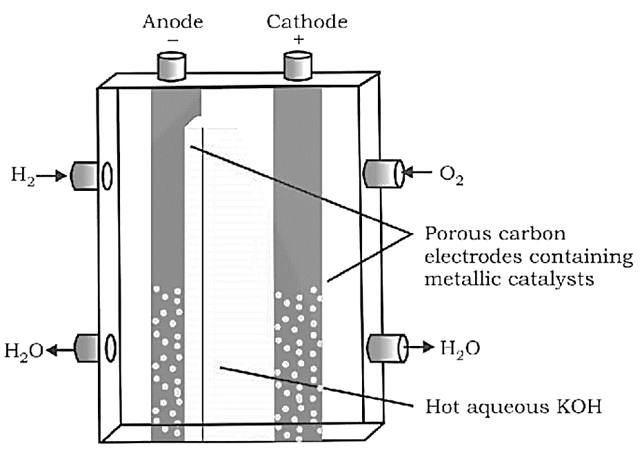
Fuel Cells

A fuel cell varies from a traditional battery in that the reactants are supplied externally from a reservoir rather than being stored inside the cell. In space vehicles, fuel cells are employed, and the two gases are supplied from external storage. The electrodes in this cell are carbon rods, and the electrolyte is $KOH$ .

Cathode: ${O_2}(g) + 2{H_2}O(l) + 4{e^ - } \to 4O{H^ - }(aq)$

Anode: $2{H_2}(g) + 4O{H^ - }(aq) \to 4{H_2}O(l) + 4{e^ - }$ 

Overall Reaction: $2{H_2}(g) + {O_2}(g) \to 2{H_2}O(l)$

Corrosion

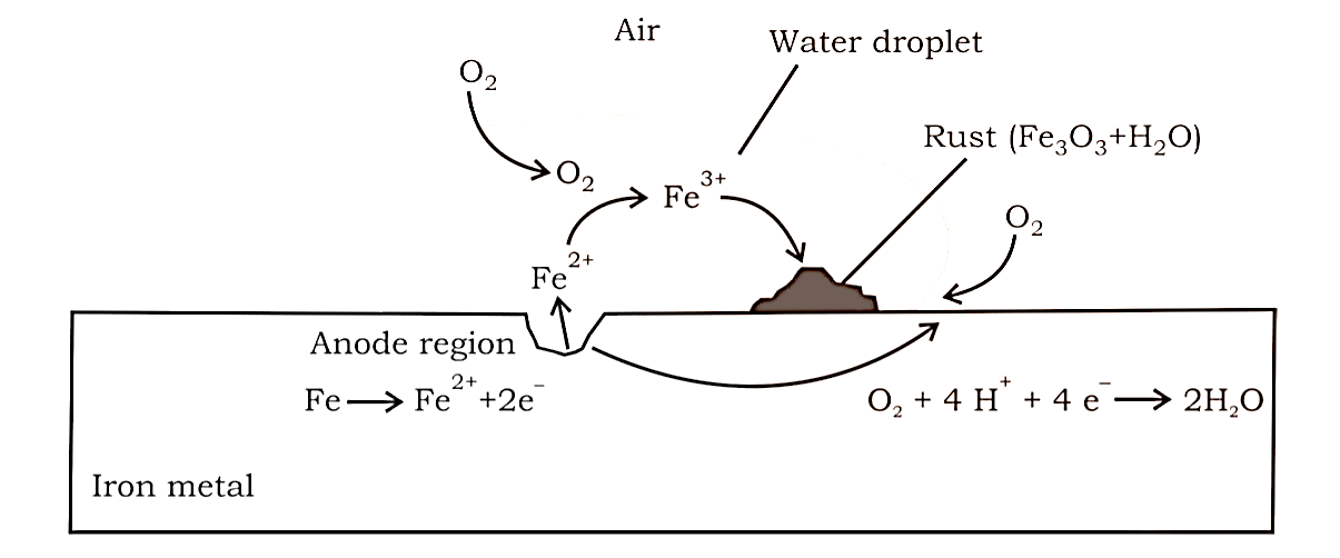
On the surface of iron or any other metal, it entails a redox process and the development of an electrochemical cell.

The oxidation of iron (anode) occurs at one point, while the reduction of oxygen to generate water occurs at another (cathode). $Fe$  is first oxidised to $F{e^{2 + }}$ , which is then converted to $F{e^{3 + }}$  in the presence of oxygen, which subsequently combines with water to generate rust, which is represented by $F{e_2}{O_3}.x{H_2}O$ .

Anode: $2Fe(s) \to 2F{e^{2 + }} + 4{e^ - }$ , ${E^ \circ } =  + 0.44\;V$ 

Cathode: ${O_2}(g) + 4{H^ + } + 4{e^ - } \to 2{H_2}O(l)$ , ${E^ \circ } = 1.23\;V$ 

Overall Reaction: $2Fe(s) + {O_2}(g) + 4{H^ + } \to 2F{e^{2 + }} + 2{H_2}O$ , $E_{Cell}^ \circ  = 1.67\;M$ 

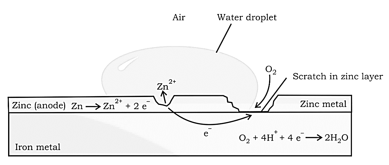
Painting or coating iron with other metals, such as zinc, helps prevent it from rusting. Galvanisation is the name for the latter procedure. Because $Zn$  has a higher potential to oxidise than iron, it is oxidised first, while iron is protected. Cathodic Protection is another name for this approach of shielding one metal by the other.

Conductance (G)

It is defined as the ease with which electric current passes through a conductor and is the reciprocal of resistance.

$G = \dfrac{1}{R}$ 

SI unit is Siemen (S).

$1\;S = 1\;oh{m^{ - 1}}(mho)$ 

Conductivity 

It is the reciprocal of resistivity $(\rho )$ .

$\kappa  = \dfrac{1}{\rho } = \dfrac{1}{R} \times \dfrac{\ell }{A} = G \times \dfrac{\ell }{A}$

Now is $l = 1\;cm$ and $A = 1\;c{m^2}$ , then $\kappa  = G$

 As a result, the conductivity of an electrolytic solution can be defined as the conductance of a $1\;cm$  long solution with a $1\;c{m^2}$  cross-sectional area.

Factors Affecting Electrolyte Conductance

Electrolyte

In a dissolved or molten form, an electrolyte is a substance that dissociates in solution to produce ions and hence conducts electricity.

Examples: $HCl,\;NaOH,\;KCl$ are strong electrolytes and $C{H_3}COOH,\;N{H_4}OH$ are weak electrolytes.

Electrolytic or ionic conductance refers to the conductance of electricity by ions present in solutions. The flow of electricity through an electrolyte solution is governed by the following factors.

1. Electrolyte Nature or Interionic Attractions: The lower the solute-solute interactions, the larger the freedom of ion mobility and the higher the conductance.

2. Ion Solvation: As the amount of solute-solvent interactions increases, the extent of solvation increases, and the electrical conductance decreases.

3. The Nature of the Solvent and its Viscosity: The larger the solvent-solvent interactions, the higher the viscosity, and the greater the solvent's resistance to ion flow, and thus the lower the electrical conductance.

4. Temperature: As the temperature of an electrolytic solution rises, solute-solute, solute-solvent, and solvent-solvent interactions diminish, causing electrolytic conductance to rise.

Measurement of Conductance

As we know, $\kappa  = \dfrac{1}{{\text{R}}} \times \dfrac{\ell }{{\text{A}}}$ 

 If we measure $l$ , $A$ , and $R$ , we can figure out what the value of $\kappa $  is. Using the ‘Wheatstones' bridge method, the resistance of the solution $R$  between two parallel electrodes is calculated.

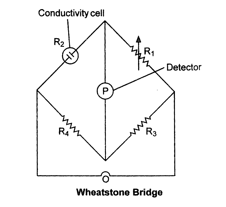
It is made up of two fixed resistances, R3 and R4, a variable resistance R1, and a conductivity cell with an unknown resistance, R2. When no current goes through the detector, the bridge is balanced. Then, in these circumstances:

$\dfrac{{{R_1}}}{{{R_2}}} = \dfrac{{{R_3}}}{{{R_4}}}$  or ${R_2} = \dfrac{{{R_1}{R_4}}}{{{R_3}}}$ 

Molar Conductivity

It's the total conducting power of all the ions created by dissolving one mole of an electrolyte between two big electrodes separated by one centimetre.

Mathematically,

\[\Lambda_{m} = \kappa \times V, \Lambda_{m} = \frac{\kappa \times V}{C}\]

where, V is the volume of solution in $c{m^3}$  containing 1 mole of electrolyte and C is the molar concentration.

Units: \[\Lambda_{m} = \frac{\kappa \times V}{C} = \frac{\text{S }cm^{-1}}{\text{mol } cm^{-1}}\]

${ = {\text{oh}}{{\text{m}}^{ - 1}}{\text{c}}{{\text{m}}^2}{\text{mo}}{{\text{l}}^{ - 1}}{\text{orSc}}{{\text{m}}^2}{\text{mo}}{{\text{l}}^{ - 1}}}$ 

Equivalent Conductivity

It is the electrical conductivity of one equivalent electrolyte placed between two big electrodes separated by one centimetre.

Mathematically:

${{{{\Lambda }}_{{\text{eq}}}} = \kappa  \times {\text{v}} = }$

${{{{\Lambda }}_{{\text{eq}}}} = \dfrac{{\kappa  \times 1000}}{{\text{N}}}}$

Where, v is the volume of solution in $c{m^3}$  containing 1 equivalent of electrolyte and N is normality.

Units:

${{{{\Lambda }}_{{\text{eq}}}} = \dfrac{{\kappa  \times 1000}}{{\text{N}}}}$

${ = \dfrac{{{\text{Sc}}{{\text{m}}^{ - 1}}}}{{{{\;equivalent\;c}}{{\text{m}}^{ - 3}}}} = \dfrac{{{\text{Oh}}{{\text{m}}^{ - 1}}{\text{c}}{{\text{m}}^2}{{\;equivalent}}{{{\;}}^{ - 1}}}}{{{\text{Sc}}{{\text{m}}^2}{{\;equivalent}}{{{\;}}^{ - 1}}}}}$

Variation of Conductivity and Molar Conductivity with Dilution

Because the number of ions per unit volume that carry the current in the solution reduces as concentration lowers, conductivity drops. With a decrease in concentration, molar conductivity rises. This is due to an increase in the total volume V of a solution containing one mole of electrolyte. The drop in $\kappa $  as a result of dilution of a solution has been found to be more than compensated by increases in its volume.

Graphical representation of the variation of ${\Lambda _m}$ vs $\sqrt c $ .

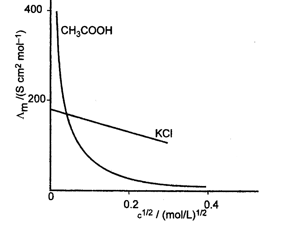
Limiting Molar Conductivity $({\Lambda _m})$ 

Limiting molar conductivity, also known as molar conductivity at infinite dilution, is the value of molar conductivity as the concentration approaches zero. In the case of a strong electrolyte, extrapolation of the ${\Lambda _m}$  vs $\sqrt c $  curve can be used to derive the molar conductivity at infinite dilution. Extrapolation of the curve, on the other hand, cannot be used to calculate the value of molar conductivity of a weak electrolyte at infinite dilution since the curve becomes practically parallel to the y-axis as concentration approaches zero.

The mathematical relationship between ${\Lambda _m}$  and $\Lambda _m^ \circ $  for a strong electrolyte was developed by Debye, Huckel and Onsagar.

In simplified form the equation can be given as:

${{t{\Lambda }}_{\text{m}}} = {{\Lambda }}_{\text{m}}^\infty  - {\text{b}}{{\text{c}}^{1/2}}$

Kohlrausch’s Law

 It asserts that an electrolyte limiting molar conductivity can be described as the total of the individual contributions of the electrolyte's anion and cation.

In general, if an electrolyte produces ${v_ + }$  cations and ${v_ - }$  anions upon dissociation, its limiting molar conductivity is given by:

${{\Lambda }}_{\text{m}}^\infty  = {{\text{v}}_ + }\lambda _ + ^ \circ  + {{\text{v}}_ - }\lambda _ - ^ \circ $

Applications of Kohlrausch’s Law

1. Calculation of molar conductivities of weak electrolyte at infinite dilution

 For example, the molar conductivity of acetic acid at infinite dilution can be calculated using the molar conductivities of strong electrolytes like $HCl$ , $C{H_3}COONa$ , and $NaCl$  at infinite dilution, as shown below.

${{\Lambda }}_{{\text{m}}\left( {{\text{C}}{{\text{H}}_3} - {\text{COOH}}} \right)}^{\text{o}} = {{\Lambda }}_{{\text{m}}\left( {{\text{C}}{{\text{H}}_3} - {\text{cooNa}}} \right)}^{\text{o}} + {{\Lambda }}_{{\text{m}}({\text{HCl}})}^{\text{o}} - {{\Lambda }}_{{\text{m}}({\text{NaCl}})}^ \circ $

2. Determination of Degree of Dissociation of Weak Electrolytes

 Degree of dissociation $\alpha  = \dfrac{{\Lambda _m^c}}{{\Lambda _m^ \circ }}$ 

3. Determination of Dissociation Constant of Weak Electrolytes:

${{\text{K}} = \dfrac{{{\text{c}}{\alpha ^2}}}{{1 - \alpha }}}$

${\alpha  = \dfrac{{{{\Lambda }}_{\text{m}}^{\text{c}}}}{{{{\Lambda }}_{\text{m}}^\infty }}}$

${{\text{K}} = \dfrac{{{\text{c}}{{\left( {{{\Lambda }}_{\text{m}}^{\text{c}}/{{\Lambda }}_{\text{m}}^\infty } \right)}^2}}}{{1 - {{\Lambda }}_{\text{m}}^c/{{\Lambda }}_{\text{m}}^\infty }} = \dfrac{{{\text{C}}{{\left( {{{\Lambda }}_{\text{m}}^{\text{c}}} \right)}^2}}}{{{{\Lambda }}_{\text{m}}^\infty \left( {{{\Lambda }}_{\text{m}}^ *  - {{\Lambda }}_{\text{m}}^{\text{c}}} \right)}}}$ 

Use of $\Delta G$ in Relating EMF values of Half Cell Reactions

When we have two half-cell reactions that produce another half-cell reaction when we combine them, their emfs cannot be mixed directly. However, thermodynamic functions such as $\Delta G$  can be added and EMF values can be connected through them in any scenario. Take a look at the three half-cell responses below:

$F{e^{2 + }} + 2{e^ - } \to Fe$ , ${E_1}$

$F{e^{3 + }} + 3{e^ - } \to Fe$ , ${E_2}$

$F{e^{3 + }} + {e^ - } \to F{e^{2 + }}$ , ${E_3}$ 

We can clearly see that subtracting the first reaction from the second yields the third reaction. However, the same relationship does not hold true for EMF values. 

That is: ${E_3} \ne {E_2} - {E_1}$ . But the $\Delta G$ values can be related according to the reactions:

${{{\Delta }}{{\text{G}}_3} = {\text{\Delta }}{{\text{G}}_2} - {{\Delta }}{{\text{G}}_1}}$

${ - {{\text{n}}_3}{\text{F}}{{\text{E}}_3} =  - {{\text{n}}_2}{\text{F}}{{\text{E}}_2} + {{\text{n}}_1}{\text{F}}{{\text{E}}_1}}$

${ - {{\text{E}}_3} =  - 3{{\text{E}}_2} + 2{{\text{E}}_1}}$

${ \Rightarrow {{\mathbf{E}}_3} = 3{{\mathbf{E}}_2} - {\mathbf{2}}{{\mathbf{E}}_1}}$ 

Formula:

1. ${\text{R}} = \rho \left( {\dfrac{\ell }{{\text{A}}}} \right) = \rho  \times {\text{Cell constant}}$

Where, $R$ = Resistance, 

$A$ = Area of cross-section of the electrodes

$\rho $ = Resistivity

2.  $\kappa  = \dfrac{1}{{\text{R}}} \times {\text{\;cell constant\;}}$

Where, $\kappa $ = Conductivity or specific conductance

3. ${{{\Lambda }}_{\text{m}}} = \dfrac{{\kappa  \times 1000}}{{\text{M}}}$

Where, ${\Lambda _m}$ = Molar conductivity 

$M$ = Molarity of the solution.

4. ${{\Lambda }}_m^\infty \left( {{A_x}{B_y}} \right) = x{{\Lambda }}_m^\infty \left( {{A^y}} \right) + y{\text{\Lambda }}_m^\infty \left( {{B^{x - }}} \right)$

5.  $\alpha  = \dfrac{{\Lambda _m^c}}{{\Lambda _m^ \circ }}$

Where, $\alpha $ = Degree of dissociation

$\Lambda _m^c$ = Molar conductivity at a given concentration

6. For a weak binary electrolyte AB

${\text{K}} = \dfrac{{{\text{c}}{\alpha ^2}}}{{1 - \alpha }} = \dfrac{{{\text{c}}{{\left( {{{\Lambda }}_{\text{m}}^{\text{c}}} \right)}^2}}}{{{{\Lambda }}_{\text{m}}^\infty \left( {{{\Lambda }}_{\text{m}}^\infty  - {{\Lambda }}_{\text{m}}^{\text{c}}} \right)}}$

Where, K is the Dissociation constant

${{\text{E}}_{{\text{edl}}}^ \circ  = {\text{E}}_{{\text{cathode}}}^ \circ  + {\text{E}}_{{\text{anode}}}^ \circ }$

${ = {{\text{E}}^ \circ }{\text{Right}} + {{\text{E}}^{\text{o}}}{\text{left}}}$

7. Nernst equation for a generation electrochemical reation

${E_{{\text{ofll}}}} = E_{{\text{cell}}}^ \circ  - \dfrac{{0.059}}{n}\log \dfrac{{{{[A]}^2}{{[B]}^b}}}{{{{[C]}^c}{{[D]}^d}}}$

8.  $\log {{\text{K}}_{\text{c}}} = \dfrac{{\text{n}}}{{0.0591}}{\text{E}}_{{\text{cell}}}^ \circ $

Where, ${K_c}$ = Equilibrium constant.

9. ${{{\Delta }}_r}{{\text{G}}^ \circ } =  - {\text{nFE}}_{{\text{cell}}}^ \circ $

${{{\Delta }}_{\text{r}}}{{\text{G}}^ \circ } =  - 2.303{\text{RT}}\log {{\text{K}}_{\text{c}}}$

${\Delta _r}{G^ \circ }$ = Standard Gibbs energy of a reaction

10. $Q = I \times t$ 

Where, $Q$ = Quantity of charge in coulombs

$I$ = Current in amperes

$t$ = Time in seconds

11. $m = Z \times I \times t$ 

Where, $m$ = mass of the substance liberated at the electrodes

$Z$ = Electrochemical equivalent

Standard Reduction Potential At 298 K. In Electrochemical Order

$\mathrm{H}_{4} \mathrm{XeO}_{6}+2 \mathrm{H}^{+}+2 \mathrm{e}^{-} \rightarrow \mathrm{XeO}_{3}+3 \mathrm{H}_{2} \mathrm{O} \quad\quad\quad\quad+3.0$

$\mathrm{~F}_{2}+2 \mathrm{e}^{-} \rightarrow 2 \mathrm{~F}^{-}  \quad\quad\quad\quad+2.87$

$\mathrm{O}_{3}+2 \mathrm{H}^{+}+2 \mathrm{e}^{-} \rightarrow \mathrm{O}_{2}+\mathrm{H}_{2} \mathrm{O} \quad\quad\quad\quad +2.07$

$\mathrm{~S}_{2} \mathrm{O}_{8}^{2-}+2 \mathrm{e}^{-} \rightarrow 2 \mathrm{SO}_{4}^{2-} \quad\quad\quad\quad +2.05$

$\mathrm{Ag}^{2+}+\mathrm{c}^{-} \rightarrow \mathrm{Ag}^{+} \quad\quad\quad\quad +1.98$

$\mathrm{Co}^{3+}+\mathrm{e}^{-} \rightarrow \mathrm{Co}^{2+} \quad\quad\quad\quad +1.81$

$\mathrm{H}_{2} \mathrm{O}_{2}+2 \mathrm{H}^{+}+2 \mathrm{e}^{-} \rightarrow 2 \mathrm{H}_{2} \mathrm{O} \quad\quad\quad\quad +1.78$

$\mathrm{Au}^{+}+\mathrm{e}^{-} \rightarrow \mathrm{Au} \quad\quad\quad\quad +1.69$

$\mathrm{~Pb}^{4+}+2 \mathrm{e}^{-} \rightarrow \mathrm{Pb}^{2+} \quad\quad\quad\quad +1.67$

$2 \mathrm{HClO}+2 \mathrm{H}^{+}+2 \mathrm{e}^{-} \rightarrow \mathrm{Cl}_{2}+2 \mathrm{H}_{2} \mathrm{O} \quad\quad\quad\quad +1.63$

$\mathrm{Ce}^{4+}+\mathrm{e}^{-} \rightarrow \mathrm{Ce}^{3+} \quad\quad\quad\quad +1.61$

$2 \mathrm{H} \mathrm{IBrO}+2 \mathrm{H}^{+}+2 \mathrm{e}^{-} \rightarrow \mathrm{Br}_{2}+2 \mathrm{H}_{2} \mathrm{O} \quad\quad\quad\quad +1.60$

$\mathrm{MnO}_{4}^{-}+8 \mathrm{H}^{+}+5 \mathrm{e}^{-} \rightarrow \mathrm{Mn}^{2+}+4 \mathrm{H}_{2} \mathrm{O} \quad\quad\quad\quad +1.51$

$\mathrm{Mn}^{3+}+\mathrm{e}^{-} \rightarrow \mathrm{Mn}^{2+} \quad\quad\quad\quad +1.51$

$\mathrm{Au}^{3+}+3 \mathrm{e}^{-} \rightarrow \mathrm{Au} \quad\quad\quad\quad +1.40$

$\mathrm{Cl}_{2}+2 \mathrm{e}^{-} \rightarrow 2 \mathrm{Cl}^{-} \quad\quad\quad\quad +1.36$

$\mathrm{Cr}_{2} \mathrm{O}_{7}^{2-}+14 \mathrm{H}^{+}+6 \mathrm{e}^{-} \rightarrow 2 \mathrm{Cr}^{3+}+7 \mathrm{H}_{2} \mathrm{O} \quad\quad\quad\quad +1.33$

$\mathrm{O}_{3}+\mathrm{H}_{2} \mathrm{O}+2 \mathrm{e}^{-} \rightarrow \mathrm{O}_{2}+2 \mathrm{OH}^{-} \quad\quad\quad\quad +1.24$

$\mathrm{O}_{2}+4 \mathrm{H}^{+} 4 \mathrm{e}^{-} \rightarrow 2 \mathrm{H}_{2} \mathrm{O} \quad\quad\quad\quad +1.23$

$\mathrm{Hg}_{2} \mathrm{SO}_{4}+2 \mathrm{e}^{-} \rightarrow 2 \mathrm{Hg}+\mathrm{SO}_{4}^{2-} \quad \quad \quad \quad +0.62$

$\mathrm{MnO}_{4}^{2-}+2 \mathrm{H}_{2} \mathrm{O}+2 \mathrm{e}^{-} \rightarrow \mathrm{MnO}_{2}+4 \mathrm{OH}^{-} \quad \quad \quad \quad +0.60$

$\mathrm{MnO}_{4}^{-}+\mathrm{e}^{-} \rightarrow \mathrm{MnO}_{4}^{2-} \quad \quad \quad \quad +0.56$

$\mathrm{I}_{2}+2 \mathrm{e}^{-} \rightarrow 2 \mathrm{I}^{-} \quad \quad \quad \quad +0.54$

$\mathrm{Cu}^{+}+\mathrm{e}^{-} \rightarrow \mathrm{Cu} \quad \quad \quad \quad +0.52$

$\mathrm{I}_{3}^{-}+2 \mathrm{e}^{-} \rightarrow 3 \mathrm{I}^{-} \quad \quad \quad \quad +0.53$

$\mathrm{NiOOH}+\mathrm{H}_{2} \mathrm{O}+\mathrm{e}^{-} \rightarrow \mathrm{Ni}(\mathrm{OH})_{2}+\mathrm{OH}^{-} \quad \quad \quad \quad +0.49$

$\mathrm{Ng}_{2} \mathrm{CrO}_{4}+2 \mathrm{e}^{-} \rightarrow 2 \mathrm{Ag}+\mathrm{CrO}_{4}^{2-} \quad \quad \quad \quad +0.45$

$\mathrm{O}_{2}+2 \mathrm{H}_{2} \mathrm{O}+4 \mathrm{e}^{-} \rightarrow 4 \mathrm{OH}^{-} \quad \quad \quad \quad +0.40$

$\mathrm{ClO}_{4}^{-}+\mathrm{H}_{2} \mathrm{O}+2 \mathrm{e}^{-} \rightarrow \mathrm{ClO}_{3}^{-}+2 \mathrm{OH}^{-} \quad \quad \quad \quad +0.36$

${\left[\mathrm{Fe}(\mathrm{CN})_{6}^{3-}+\mathrm{e}^{-} \rightarrow\left[\mathrm{Fe}(\mathrm{CN})_{6}\right]^{+}\right.} \quad \quad \quad \quad +0.36$

$\mathrm{Cu}^{2+}+2 \mathrm{e}^{-} \rightarrow \mathrm{Cu} \quad \quad \quad \quad +0.34$

$\mathrm{Hg}_{2} \mathrm{Cl}_{2}+2 \mathrm{e}^{-} \rightarrow 2 \mathrm{Hg}+2 \mathrm{Cl}^{-} \quad \quad \quad \quad +0.27$

$\mathrm{AgCl}+\mathrm{e}^{-} \rightarrow \mathrm{Ag}+\mathrm{Cl}^{-} \quad \quad \quad \quad +0.22$

$\mathrm{Bi}+3 \mathrm{e}^{-} \rightarrow \mathrm{Bi} \quad \quad \quad \quad +0.20$

$\mathrm{Cu}^{2+}+\mathrm{e}^{-} \rightarrow \mathrm{Cu}^{+} \quad \quad \quad \quad +0.16$

$\mathrm{Sn}^{4+}+2 \mathrm{e}^{-} \rightarrow \mathrm{Sn}^{2+} \quad \quad \quad \quad +0.15$

$\mathrm{AgBr}+\mathrm{e}^{-} \rightarrow \mathrm{Ag}+\mathrm{Br}^{-} \quad \quad \quad \quad +0.07$

$\mathrm{ClO}_{4}^{-}+2 \mathrm{H}^{+}+2 \mathrm{e}^{-} \rightarrow \mathrm{ClO}_{3}^{-}+\mathrm{H}_{2} \mathrm{O} \quad \quad \quad \quad +1.23$

$\mathrm{MNO}_{2}+4 \mathrm{H}^{+}+2 \mathrm{e}^{-} \rightarrow \mathrm{Mn}^{2+}+2 \mathrm{H}_{2} \mathrm{O} \quad \quad \quad \quad +1.23$

$\mathrm{Br}_{2}+2 \mathrm{e}^{-} \rightarrow 2 \mathrm{Br}^{-} \quad \quad \quad \quad +1.09$

$\mathrm{Pu}^{4+}+\mathrm{e}^{-} \rightarrow \mathrm{Pu}^{3+} \quad \quad \quad \quad +0.97$

$\mathrm{NO}_{3}^{-}+4 \mathrm{H}^{+}+3 \mathrm{e}^{-} \rightarrow \mathrm{NO}+2 \mathrm{H}_{2} \mathrm{O} \quad \quad \quad \quad +0.96$

$2 \mathrm{Hg}^{2+}+2 \mathrm{e}^{-} \rightarrow \mathrm{Hg}_{2}^{2+} \quad \quad \quad \quad +0.92$

$\mathrm{ClO}^{-}+\mathrm{H}_{2} \mathrm{O}+2 \mathrm{e}^{-} \rightarrow \mathrm{Cl}^{-}+2 \mathrm{OH}^{-} \quad \quad \quad \quad +0.89$

$\mathrm{Hg}^{2+}+2 \mathrm{e}^{-} \rightarrow \mathrm{Hg} \quad \quad \quad \quad +0.86$

$\mathrm{NO}_{3}^{-}+2 \mathrm{H}^{+}+\mathrm{e}^{-} \rightarrow \mathrm{NO}_{2}+\mathrm{H}_{2} \mathrm{O} \quad \quad \quad \quad +0.80$

$\mathrm{Ag}^{+}+\mathrm{e}^{-} \rightarrow \mathrm{Ag} \quad \quad \quad \quad +0.80$

$\mathrm{Hg}_{2}^{2+}+2 \mathrm{e}^{-} \rightarrow 2 \mathrm{Hg} \quad \quad \quad \quad +0.79$

$\mathrm{Fe}^{3+}+\mathrm{e}^{-} \rightarrow \mathrm{Fe}^{2+} \quad \quad \quad \quad +0.77$

$\mathrm{BrO}^{-}+\mathrm{H}_{2} \mathrm{O}+2 \mathrm{e}^{-} \rightarrow \mathrm{Br}^{-}+2 \mathrm{OH}^{-} \quad \quad \quad \quad +0.76$

$\mathrm{Ti}^{4+}+\mathrm{e}^{-} \rightarrow \mathrm{Ti}^{3+} \quad \quad \quad \quad 0.00  2 \mathrm{H}^{+}+2 \mathrm{e}^{-} \rightarrow \mathrm{H}_{2} \quad \quad \quad \quad 0, \text { by definition }$

$\mathrm{Fe}^{3-}+3 \mathrm{e}^{-} \rightarrow \mathrm{Fe} \quad \quad \quad \quad -0.04$

$\mathrm{O}_{2} \mathrm{H}_{2} \mathrm{O}+2 \mathrm{e}^{-} \rightarrow \mathrm{HO}_{2}^{-}+\mathrm{OH}^{-} \quad \quad \quad \quad -0.08$

$\mathrm{~Pb}^{2+}+2 \mathrm{e}^{-} \rightarrow \mathrm{Pb} \quad \quad \quad \quad -0.13$

$\mathrm{In}^{+}+\mathrm{e}^{-} \rightarrow \mathrm{In} \quad \quad \quad \quad -0.14$

$\mathrm{Sn}^{2+}+2 \mathrm{e}^{-} \rightarrow \mathrm{Sn} \quad \quad \quad \quad -0.14$

$\mathrm{AgI}+\mathrm{e}^{-} \rightarrow \mathrm{Ag}+\mathrm{F}^{-} \quad \quad \quad \quad -0.15$

$\mathrm{Ni}^{2+}+2 \mathrm{e}^{-} \rightarrow \mathrm{Ni} \quad \quad \quad \quad -0.23$

$\mathrm{Co}^{2+}+2 \mathrm{e}^{-} \rightarrow \mathrm{Co} \quad \quad \quad \quad -0.28$

$\mathrm{In}^{3+}+3 \mathrm{e}^{-} \rightarrow \mathrm{In} \quad \quad \quad \quad -0.34$ 

$\mathrm{Tl}^{+}\mathrm{e}^{-} \rightarrow \mathrm{Tl} \quad \quad \quad \quad -0.34$

$\mathrm{PbSO}_{4}+2 \mathrm{e}^{-} \rightarrow \mathrm{Pb}+\mathrm{SO}_{4}^{2-} \quad \quad \quad \quad -0.36$

$\mathrm{Ti}^{3+}+\mathrm{e}^{-} \rightarrow \mathrm{Ti}^{2+} \quad \quad \quad \quad -0.37$

$\mathrm{Cd}^{2+}+2 \mathrm{e}^{-} \rightarrow \mathrm{Cd} \quad \quad \quad \quad -0.40$

$\mathrm{In}^{2+}+\mathrm{e}^{-} \rightarrow \mathrm{In}^{+} \quad \quad \quad \quad -0.40$

$\mathrm{Cr}^{3+}+\mathrm{e}^{-} \rightarrow \mathrm{Cr}^{2+} \quad \quad \quad \quad -0.41$

$\mathrm{Fe}^{2+}+2 \mathrm{e}^{-} \rightarrow \mathrm{Fe} \quad \quad \quad \quad -0.44$

$\mathrm{In}^{3+}+2 \mathrm{e}^{-} \rightarrow \mathrm{In}^{+} \quad \quad \quad \quad -0.44$

$\mathrm{~S}+2 \mathrm{e}^{-} \rightarrow \mathrm{S}^{2-} \quad \quad \quad \quad -0.48$

$\mathrm{In}^{3+}+\mathrm{e}^{-} \rightarrow \mathrm{In}^{2+} \quad \quad \quad \quad -0.49$

$\mathrm{U}^{4+}+\mathrm{e}^{-} \rightarrow \mathrm{U}^{3+} \quad \quad \quad \quad -0.61$

$\mathrm{Cr}^{3+}+3 \mathrm{e}^{-} \rightarrow \mathrm{Cr} \quad \quad \quad \quad -0.74$

$\mathrm{Zn}^{2+}+2 \mathrm{e}^{-} \rightarrow \mathrm{Zn} \quad \quad \quad \quad -0.76$

$\mathrm{Cd}(\mathrm{OH})_{2}+2 \mathrm{e}^{-} \rightarrow \mathrm{Cd}+2 \mathrm{OH}^{-} \quad \quad \quad \quad -0.81$

$2 \mathrm{H}_{2} \mathrm{O}+2 \mathrm{e}^{-} \rightarrow \mathrm{H}_{2}+2 \mathrm{OH}^{-} \quad \quad \quad \quad -0.83$

$\mathrm{Cr}^{2+}+2 \mathrm{e}^{-} \rightarrow \mathrm{Cr} \quad \quad \quad \quad -0.91$

$\mathrm{Mn}^{2+}+2 \mathrm{e}^{-} \rightarrow \mathrm{Mn} \quad \quad \quad \quad -1.18$

$\mathrm{V}^{2+}+2 \mathrm{e}^{-} \rightarrow \mathrm{V} \quad \quad \quad \quad -1.19$ 

$\mathrm{Ti}^{2+}+2 \mathrm{e}^{-} \rightarrow \mathrm{Ti} \quad \quad \quad \quad -1.63$ 

$\mathrm{Al}^{3+}+3 \mathrm{e}^{-} \rightarrow \mathrm{Al} \quad \quad \quad \quad -1.66$ 

$\mathrm{U}^{3+}+3 \mathrm{e}^{-} \rightarrow \mathrm{U} \quad \quad \quad \quad -1.79$ 

$\mathrm{Sc}^{3+}+3 \mathrm{e}^{-} \rightarrow \mathrm{Sc} \quad \quad \quad \quad -2.09$ 

$\mathrm{Mg}^{2+}+2 \mathrm{e}^{-} \rightarrow \mathrm{Mg} \quad \quad \quad \quad -2.36$ 

$\mathrm{Ce}^{3+}+3 \mathrm{e}^{-} \rightarrow \mathrm{Ce} \quad \quad \quad \quad -2.48$ 

$\mathrm{La}^{3+}+3 \mathrm{e}^{-} \rightarrow \mathrm{La} \quad \quad \quad \quad -2.52$ 

$\mathrm{Na}^{+}+\mathrm{e}^{-} \rightarrow \mathrm{Na} \quad \quad \quad \quad -2.71$ 

$\mathrm{Ca}^{2+}+2 \mathrm{e}^{-} \rightarrow \mathrm{Ca} \quad \quad \quad \quad -2.87$ 

$\mathrm{Sr}^{2+}+2 \mathrm{e}^{-} \rightarrow \mathrm{Sr} \quad \quad \quad \quad -2.89$ 

$\mathrm{Ba}^{2+}+2 \mathrm{e}^{-} \rightarrow \mathrm{Ba} \quad \quad \quad \quad -2.91$

$\mathrm{Ra}^{2+}+2 \mathrm{e}^{-} \rightarrow \mathrm{Ra} \quad \quad \quad \quad -2.92$ 

$\mathrm{Cs}^{+}+\mathrm{e}^{-} \rightarrow \mathrm{Cs} \quad \quad \quad \quad -2.92$ 

$\mathrm{Rb}^{+}+\mathrm{e}^{-} \rightarrow \mathrm{Rb} \quad \quad \quad \quad -2.93$ 

$\mathrm{~K}^{+}+\mathrm{e}^{-} \rightarrow \mathrm{K} \quad \quad \quad \quad -2.93$ 

$\mathrm{Li}^{+}+\mathrm{e}^{-} \rightarrow \mathrm{Li} \quad \quad \quad \quad -3.05$

Reduction Potential in Alphabetical Order: 

$\mathrm{Ag}^{+}+\mathrm{e}^{-} \rightarrow \mathrm{Ag}$

$\mathrm{Ag}^{2+}+\mathrm{e}^{-} \rightarrow \mathrm{Ag}^{+}$

$\mathrm{AgBr}+\mathrm{e}^{-} \rightarrow \mathrm{Ag}+\mathrm{Br}^{-}$

$\mathrm{AgCl}+\mathrm{e}^{-} \rightarrow \mathrm{Ag}+\mathrm{Cl}^{-}$

$\mathrm{Ag}_{2} \mathrm{CrO}_{4}+2 \mathrm{e}^{-} \rightarrow 2 \mathrm{Ag}+\mathrm{CrO}_{4}^{2-}$

$\mathrm{AgF}+\mathrm{e}^{-} \rightarrow \mathrm{Ag}+\mathrm{F}^{-}$

$\mathrm{Agl}+\mathrm{e}^{-} \rightarrow \mathrm{Ag}+\mathrm{I}^{-}$

$\mathrm{Al}^{3+}+3 \mathrm{e}^{-} \rightarrow \mathrm{Al}$

$\mathrm{Au}^{+}+\mathrm{e}^{-} \rightarrow \mathrm{Au}$

$\mathrm{Au}^{3+}+3 \mathrm{e}^{-} \rightarrow \mathrm{Au}$

$\mathrm{Ba}^{2+}+2 \mathrm{e}^{-} \rightarrow \mathrm{Ba}$

$\mathrm{Be}^{2+}+2 \mathrm{e}^{-} \rightarrow \mathrm{Be}$

$\mathrm{Bi}^{-3+}+3 \mathrm{e}^{-} \rightarrow \mathrm{Bi}$

$\mathrm{Br}_{2}+2 \mathrm{e}^{-} \rightarrow 2 \mathrm{Br}^{-}$

$\mathrm{BrO}^{-}+\mathrm{H}_{2} \mathrm{O}+2 \mathrm{e}^{-} \rightarrow \mathrm{Br}^{-}+2 \mathrm{OH}^{-}$

$\mathrm{Ca}^{2+}+2 \mathrm{e}^{-} \rightarrow \mathrm{Ca} \quad \quad \quad \quad -2.87$

$\mathrm{Cd}(\mathrm{OH})_{2}+2 \mathrm{e}^{-} \rightarrow \mathrm{Cd}+2 \mathrm{OH}^{-} \quad \quad \quad \quad -0.81$

$\mathrm{Cd}^{2+}+2 \mathrm{e}^{-} \rightarrow \mathrm{Cd} \quad \quad \quad \quad -0.40$

$\mathrm{Ce}^{3+}+3 \mathrm{e}^{-} \rightarrow \mathrm{Ce} \quad \quad \quad \quad -2.48$

$\mathrm{Ce}^{4+}+\mathrm{e}^{-} \rightarrow \mathrm{Ce}^{3+} \quad \quad \quad \quad +1.61$

$\mathrm{Cl}_{2}+2 \mathrm{e}^{-} \rightarrow 2 \mathrm{Cl}^{-} \quad \quad \quad \quad +1.36$

$\mathrm{ClO}^{-}+\mathrm{H}_{2} \mathrm{O}+2 \mathrm{e}^{-} \rightarrow \mathrm{Cl}^{-}+2 \mathrm{OH}^{-} \quad \quad \quad \quad +0.89$

$\mathrm{ClO}_{4}^{-}+2 \mathrm{H}^{+}+2 \mathrm{e}^{-} \rightarrow \mathrm{ClO}_{3}^{-}+\mathrm{H}_{2} \mathrm{O} \quad \quad \quad \quad +1.23$

$\mathrm{ClO}_{4}^{-}+\mathrm{H}_{2} \mathrm{O}+2 \mathrm{e}^{-} \rightarrow \mathrm{ClO}_{3}^{-}+2 \mathrm{OH}^{-} \quad \quad \quad \quad +0.36$

$\mathrm{Co}^{2+}+2 \mathrm{e}^{-} \rightarrow \mathrm{Co} \quad \quad \quad \quad -0.28$

$\mathrm{Co}^{3+}+\mathrm{e}^{-} \rightarrow \mathrm{Co}^{2+} \quad \quad \quad \quad +1.81$

$\mathrm{Cr}^{2+}+2 \mathrm{e}^{-} \rightarrow \mathrm{Cr} \quad \quad \quad \quad -0.91$

$\mathrm{Cr}_{2} \mathrm{O}_{7}^{2-}+14 \mathrm{H}^{+}+6 \mathrm{e}^{-} \rightarrow 2 \mathrm{Cr}^{3+}+7 \mathrm{H}_{2} \mathrm{O} \quad \quad \quad \quad +1.33$

$\mathrm{Cr}^{3+}+3 \mathrm{e}^{-} \rightarrow \mathrm{Cr} \quad \quad \quad \quad -0.74$

$\mathrm{Cr}^{3+}+\mathrm{e}^{-} \rightarrow \mathrm{Cr}^{2+} \quad \quad \quad \quad -0.41$

$\mathrm{Cs}^{+} \mathrm{e}^{-} \rightarrow \mathrm{Cs} \quad \quad \quad \quad -2.92$

$\mathrm{Cu}^{+}+\mathrm{e}^{-} \rightarrow \mathrm{Cu} \quad \quad \quad \quad +0.52$

$\mathrm{Cu}^{2+}+2 \mathrm{e}^{-} \rightarrow \mathrm{Cu} \quad \quad \quad \quad +0.34$

$\mathrm{Cu}^{2+}+\mathrm{e}^{-} \rightarrow \mathrm{Cu}^{+} \quad \quad \quad \quad +0.16$

$\mathrm{~F}_{2}+2 \mathrm{e}^{-} \rightarrow 2 \mathrm{~F}^{-} \quad \quad \quad \quad +2.87$

$\mathrm{Fe}^{2+}+2 \mathrm{e}^{-} \rightarrow \mathrm{Fe} \quad \quad \quad \quad -0.44$

$\mathrm{Fe}^{3+}+3 \mathrm{e}^{-} \rightarrow \mathrm{Fe} \quad \quad \quad \quad -0.04$

$\mathrm{Fe}^{3+}+\mathrm{e}^{-} \rightarrow \mathrm{Fe}^{2+} \quad \quad \quad \quad +0.77$

${\left[\mathrm{Fe}(\mathrm{CN})_{6}\right]^{3}+\mathrm{e}^{-} \rightarrow\left[\mathrm{Fe}(\mathrm{CN})_{6}\right]^{+}} \quad \quad \quad \quad +0.36$

$2 \mathrm{H}^{+}+2 \mathrm{e}^{-} \rightarrow \mathrm{H}_{2} \quad \quad \quad \quad 0, \text { by definition }$

$2 \mathrm{H}_{2} \mathrm{O}+2 \mathrm{e}^{-} \rightarrow \mathrm{H}_{2}+2 \mathrm{OH}^{-} \quad \quad \quad \quad -0.83$

$2 \mathrm{HBrO}+2 \mathrm{H}^{+}+2 \mathrm{e}^{-} \rightarrow \mathrm{Br}_{2}+2 \mathrm{H}_{2} \mathrm{O} \quad \quad \quad \quad +1.60$

$2 \mathrm{HClO}+2 \mathrm{H}^{+}+2 \mathrm{e}^{-} \rightarrow \mathrm{Cl}_{2}+2 \mathrm{H}_{2} \mathrm{O} \quad \quad \quad \quad +1.63$

$\mathrm{H}_{2} \mathrm{O}_{2}+2 \mathrm{H}^{+}+2 \mathrm{e}^{-} \rightarrow 2 \mathrm{H}_{2} \mathrm{O} \quad \quad \quad \quad +1.78$

$\mathrm{H}_{4} \mathrm{XeO}_{6}+2 \mathrm{H}^{+}+2 \mathrm{e}^{-} \rightarrow \mathrm{XeO}_{3}+3 \mathrm{H}_{2} \mathrm{O} \quad \quad \quad \quad +3.0$

$\mathrm{MnO}_{4}^{-}+2 \mathrm{H}_{2} \mathrm{O}+2 \mathrm{e}^{-} \rightarrow \mathrm{MnO}_{2}+4 \mathrm{OH}^{-} \quad \quad \quad \quad +0.60$

$\mathrm{Na}^{-}+\mathrm{e}^{-} \rightarrow \mathrm{Na} \quad \quad \quad \quad -2.71$

$\mathrm{Ni}^{2+}+2 \mathrm{e}^{-} \rightarrow \mathrm{Ni} \quad \quad \quad \quad -0.23$

$\mathrm{NiOOH}+\mathrm{H}_{2} \mathrm{O}+\mathrm{e}^{-} \rightarrow \mathrm{Ni}(\mathrm{OH})_{2}+\mathrm{OH}^{-} \quad \quad \quad \quad +0.49$

$\mathrm{NO}_{3}^{-}+2 \mathrm{H}^{+}+\mathrm{e}^{-} \rightarrow \mathrm{NO}_{2}+\mathrm{H}_{2} \mathrm{O} \quad \quad \quad \quad -0.80$

$\mathrm{NO}_{3}^{-}+4 \mathrm{H}^{+}+3 \mathrm{e}^{-} \rightarrow \mathrm{NO}+2 \mathrm{H}_{2} \mathrm{O} \quad \quad \quad \quad +0.96$

$\mathrm{NO}_{3}^{-}+\mathrm{H}_{2} \mathrm{O}+2 \mathrm{e}^{-} \rightarrow \mathrm{NO}_{2}^{-}+2 \mathrm{OH}^{-} \quad \quad \quad \quad +0.10$

$\mathrm{O}_{2}+2 \mathrm{H}_{2} \mathrm{O}+4 \mathrm{e}^{-} \rightarrow 4 \mathrm{OH}^{-} \quad \quad \quad \quad +0.40$

$\mathrm{O}_{2}+4 \mathrm{H}^{+}+4 \mathrm{e}^{-} \rightarrow 2 \mathrm{H}_{2} \mathrm{O} \quad \quad \quad \quad +1.23$

$\mathrm{O}_{2}+\mathrm{e}^{-} \rightarrow \mathrm{O}_{2}^{-} \quad \quad \quad \quad -0.56$

$\mathrm{O}_{2}+\mathrm{H}_{2} \mathrm{O}+2 \mathrm{e}^{-} \rightarrow \mathrm{HO}_{2}^{-}+\mathrm{OH}^{-} \quad \quad \quad \quad -0.08$

$\mathrm{O}_{3}+2 \mathrm{H}^{+}+2 \mathrm{e}^{-} \rightarrow \mathrm{O}_{2}+\mathrm{H}_{2} \mathrm{O} \quad \quad \quad \quad +2.07$

$\mathrm{O}_{3}+\mathrm{H}_{2} \mathrm{O}+2 \mathrm{e}^{-} \rightarrow \mathrm{O}_{2}+2 \mathrm{OH}^{-} \quad \quad \quad \quad +1.24$

$\mathrm{H}_{4} \mathrm{XeO}_{6}+2 \mathrm{H}^{+}+2 \mathrm{e}^{-} \rightarrow \mathrm{XeO}_{3}+3 \mathrm{H}_{2} \mathrm{O} \quad \quad \quad \quad +3.0$

$\mathrm{Hg}_{2}^{2+}+2 \mathrm{e}^{-} \rightarrow 2 \mathrm{Hg} \quad \quad \quad \quad +0.79$

$\mathrm{Hg}_{2} \mathrm{Cl}_{2}+2 \mathrm{e}^{-} \rightarrow 2 \mathrm{Hg}+2 \mathrm{Cl}^{-} \quad \quad \quad \quad +0.27$

$\mathrm{Hg}^{2+}+2 \mathrm{e}^{-} \rightarrow \mathrm{Hg} \quad \quad \quad \quad +0.86$

$2 \mathrm{Hg}^{2+}+2 \mathrm{e}^{-} \rightarrow \mathrm{Hg}_{2}^{2+} \quad \quad \quad \quad +0.92$

$\mathrm{Hg}_{2} \mathrm{SO}_{4}+2 \mathrm{e}-\rightarrow 2 \mathrm{Hg}+\mathrm{SO}_{4}^{2-} \quad \quad \quad \quad +0.62$

$\mathrm{I}_{2}+2 \mathrm{e}^{-} \rightarrow 2 \mathrm{I}^{-} \quad \quad \quad \quad +0.54$

$\mathrm{I}_{3}^{-}+2 \mathrm{e}^{-} \rightarrow 3 \mathrm{I}^{-} \quad \quad \quad \quad +0.53$

$\mathrm{In}^{+}+\mathrm{e}^{-} \rightarrow \mathrm{In} \quad \quad \quad \quad -0.14$

$\mathrm{In}^{2+}+\mathrm{e}^{-} \rightarrow \mathrm{In}^{+} \quad \quad \quad \quad -0.40$

$\mathrm{In}^{3+}+2 \mathrm{e}^{-} \rightarrow \mathrm{In}^{+} \quad \quad \quad \quad -0.44$

$\mathrm{In}^{3+}+3 \mathrm{e}^{-} \rightarrow \mathrm{In} \quad \quad \quad \quad -0.34$

$\mathrm{In}^{3+}+\mathrm{c}^{-} \rightarrow \mathrm{In}^{2+} \quad \quad \quad \quad -0.49$

$\mathrm{~K}^{+}+\mathrm{e}^{-} \rightarrow \mathrm{K} \quad \quad \quad \quad -2.93$

$\mathrm{La}^{3+}+3 \mathrm{e}^{-} \rightarrow \mathrm{La} \quad \quad \quad \quad -2.52$

$\mathrm{Li}+\mathrm{e}^{-} \rightarrow \mathrm{Li} \quad \quad \quad \quad -3.05$

$\mathrm{Mg}^{2+}+2 \mathrm{e}^{-} \rightarrow \mathrm{Mg} \quad \quad \quad \quad -2.36$

$\mathrm{Mn}^{2+}+2 \mathrm{e}^{-} \rightarrow \mathrm{M} \quad \quad \quad \quad -1.18$

$\mathrm{Mn}^{3+}+\mathrm{e}^{-} \rightarrow \mathrm{Mn}^{2+} \quad \quad \quad \quad +1.51$

$\mathrm{MnO}_{2}+4 \mathrm{H}^{+}+2 \mathrm{e}^{-} \rightarrow \mathrm{Mn}^{2+}+2 \mathrm{H}_{2} \mathrm{O} \quad \quad \quad \quad +1.23$

$\mathrm{MnO}_{4}^{-}+8 \mathrm{H}^{+}+5 \mathrm{e}^{-} \rightarrow \mathrm{Mn}^{2+}+4 \mathrm{H}_{2} \mathrm{O} \quad \quad \quad \quad +1.51$

$\mathrm{MnO}_{4}^{-}+\mathrm{e}^{-} \rightarrow \mathrm{MnO}_{4}^{2-} \quad \quad \quad \quad +0.56$

$\mathrm{O}_{3}+\mathrm{H}_{2} \mathrm{O}+2 \mathrm{e}^{-} \rightarrow \mathrm{O}_{2}+2 \mathrm{OH}^{-} \quad \quad \quad \quad +1.24$

$\mathrm{~Pb}^{2+}+2 \mathrm{e}^{-} \rightarrow \mathrm{Pb} \quad \quad \quad \quad -0.13$

$\mathrm{~Pb}^{4+}+2 \mathrm{e}^{-} \rightarrow \mathrm{Pb}^{2+} \quad \quad \quad \quad +1.67$

$\mathrm{PbSO}_{4}+2 \mathrm{e}^{-} \rightarrow \mathrm{Pb}+\mathrm{SO}_{4}^{2-} \quad \quad \quad \quad -0.36$

$\mathrm{Pt}^{2+}+2 \mathrm{e}^{-} \rightarrow \mathrm{Pt} \quad \quad \quad \quad +1.20$

$\mathrm{Pu}^{4+}+\mathrm{e}^{-} \rightarrow \mathrm{Pu}^{3+} \quad \quad \quad \quad +0.97$

$\mathrm{Ra}^{2+}+2 \mathrm{e}^{-} \rightarrow \mathrm{Ra} \quad \quad \quad \quad -2.92$

$\mathrm{Rb}^{+}+\mathrm{e}^{-} \rightarrow \mathrm{Rb} \quad \quad \quad \quad -2.93$

$\mathrm{~S}+2 \mathrm{e}^{-} \rightarrow \mathrm{S}^{2-} \quad \quad \quad \quad -0.48$

$\mathrm{~S}_{2} \mathrm{O}_{8}^{2-}+2 \mathrm{e}^{-} \rightarrow 2 \mathrm{SO}_{4}^{2-} \quad \quad \quad \quad +2.05$

$\mathrm{SC}^{3+}+3 \mathrm{e}^{-} \rightarrow \mathrm{Sc} \quad \quad \quad \quad -2.09$

$\mathrm{Sn}^{2+}+2 \mathrm{e}^{-} \rightarrow \mathrm{Sn} \quad \quad \quad \quad -0.14$

$\mathrm{Sn}^{4+}+2 \mathrm{e}^{-} \rightarrow \mathrm{Sn}^{2+} \quad \quad \quad \quad +0.15$

$\mathrm{Sr}^{2+}+2 \mathrm{e}^{-} \rightarrow \mathrm{Sr} \quad \quad \quad \quad -2.89$

$\mathrm{Ti}^{2+}+2 \mathrm{e}^{-} \rightarrow \mathrm{Ti} \quad \quad \quad \quad -1.63$

$\mathrm{Ti}^{3+}+\mathrm{e}^{-} \rightarrow \mathrm{Ti}^{2+} \quad \quad \quad \quad -0.37$

$\mathrm{Ti}^{4+}+\mathrm{e}^{-} \rightarrow \mathrm{Ti}^{3+} \quad \quad \quad \quad 0.00$

$\mathrm{Tl}^{+}+\mathrm{e}^{-} \rightarrow \mathrm{Tl} \quad \quad \quad \quad -0.34$

$\mathrm{U}^{3+}+3 \mathrm{e}^{-} \rightarrow \mathrm{U} \quad \quad \quad \quad -1.79$

$\mathrm{U}^{4+}+\mathrm{e}^{-} \rightarrow \mathrm{U}^{3+} \quad \quad \quad \quad -0.61$

$\mathrm{~V}^{2+}+2 \mathrm{e}^{-} \rightarrow \mathrm{V} \quad \quad \quad \quad -1.19$

$\mathrm{~V}^{3+}+\mathrm{e}^{-} \rightarrow \mathrm{V}^{2+} \quad \quad \quad \quad -0.26$

$\mathrm{Zn}^{2+}+2 \mathrm{e}-\rightarrow \mathrm{Zn} \quad \quad \quad \quad -0.76$

Some Important Questions on Electrochemistry

1. What is the meaning of the negative sign in the expression $\dfrac{E_0 Zn^{2+}}{Zn} = – 0.76 V$?

Ans. The negative sign in the given expression implies that Zn is more reactive than hydrogen or that it is a stronger reducing agent than hydrogen. Zinc will be oxidised to $Zn^{2+}$ ions, while the $H^+$ ions will get reduced to hydrogen in a cell that contains a zinc electrode and a standard hydrogen electrode present in two half-cells.

2. What are the conditions under which $E_0$ cell = 0 and $\Delta rG_0 = 0$?

Ans. When at equilibrium, $E_0$cell = 0 and $\Delta rG_0 = 0$.

3. Can we measure the absolute electrode potential of an electrode?

Ans. No, it is not possible to measure the absolute potential of an electrode since the half-cell that contains a single electrode cannot work on its own, it can only work in combination with another half-cell.

Class 12 Chemistry Chapter 2: Details, Formulas and Concepts.

1. Nernst Equation: This equation relates the equilibrium potential of an electrochemical cell to the concentrations of the reactants and products involved. It's given as:

\[ E = E^\circ - \dfrac{0.0592}{nlog Q}\]

2. Gibbs Free Energy Change (ΔG): In electrochemistry, this concept is crucial as it determines whether a reaction is spontaneous or not. The relationship between Gibbs free energy change, cell potential, and temperature is given by:\[ \Delta G = -nFE \]

Class 12 Chemistry Chapter 2 Important Topics and Subtopics Covered 

Importance of Revision Notes for Class 12 Chemistry Chapter 2

• Summarises Key Points: Condenses important concepts for quick review.

• Saves Time: Provides a fast way to revise before exams.

• Highlights Essentials: Focuses on crucial topics and definitions.

• Improves Memory: Helps in better retention of information.   

• Enhances Exam Prep: Targets weak areas for more effective study.

• Clarifies Concepts: Simplifies complex ideas for easier understanding.

• Includes Visuals: Uses diagrams and charts for better grasp.

• Boosts Confidence: Prepares students thoroughly for exams.

Tips for Learning the Class 12 Chemistry Chapter 2 

1. Focus on core processes with illustrations and examples.

2. Draw and label diagrams for clarity. 

3. Create summaries of each process.

4. Connect concepts to everyday examples.

5. Solve past exam questions to test understanding.

6. Explain concepts to others to reinforce learning.

7. Revisit material frequently to retain information.

8. Utilise platforms like Vedantu for additional support.

Conclusion

Vedantu's Electrochemistry Class 12 Revision Notes for CBSE Chemistry Chapter 2 provides a comprehensive and effective resource for students studying this topic. The Electrochemistry Revision notes cover all the important concepts outlined in the NCERT textbook, ensuring that students have a clear understanding of electrochemistry. Vedantu's notes are well-structured and easy to follow, making it easier for students to grasp complex concepts and solve problems. 

Related Study Materials for Class 12 Chapter 2 Electrochemistry

Revision Notes Links for Class 12 Chemistry Revision Notes

Related Study Material Links for Class 12 Chemistry