Inverse Trigonometric Functions Class 12 Notes: CBSE Maths Chapter 2

Domain and Range of all Inverse Trigonometric Functions

• We must note that inverse trigonometric functions cannot be expressed in terms of trigonometric functions as their reciprocals. For example, ${{\sin }^{-1}}x\ne \dfrac{1}{\sin x}$.

• The principal value of a trigonometric function is that value which lies in the range of principal branch.

• The functions \[{{\sin }^{-1}}x\text{  }\!\!\And\!\!\text{  }{{\tan }^{-1}}x\] are increasing functions in their domain.

• The functions \[{{\cos }^{-1}}x\text{  }\!\!\And\!\!\text{  }{{\cot }^{-1}}x\] are decreasing functions in over domain.

Graphs of Inverse Trigonometric Functions

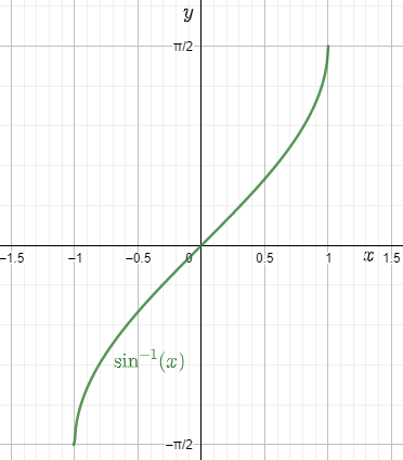
a) Graph of ${{\sin }^{-1}}x$ is shown below,

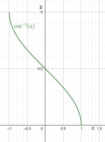
b) Graph of ${{\cos }^{-1}}x$ is shown below,

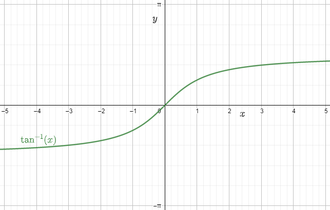
c) Graph of ${{\tan }^{-1}}x$ is shown below,

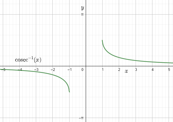
d) Graph of $\cos e{{c}^{-1}}x$ is shown below,

e) Graph of ${{\sec }^{-1}}x$ is shown below,

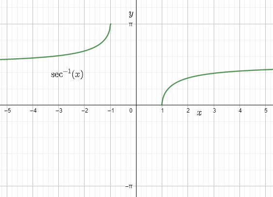
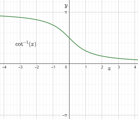
f) Graph of ${{\cot }^{-1}}x$ is shown below,

Properties of Inverse Trigonometric Functions

1. Property I

(a). \[{{\sin }^{-1}}\left( \dfrac{1}{x} \right)=\cos e{{c}^{-1}}x\], for all \[x\in \left( -\infty ,1 \right]\cup \left[ 1,\infty  \right)\]

Let us prove this by considering \[\cos e{{c}^{-1}}x=\theta \] ……(i)

Taking \[\cos ec\] on both sides,

\[x=\cos ec\theta \]

Using reciprocal identity,

\[\Rightarrow \dfrac{1}{x}=\sin \theta \]

\[\left\{ \because x\in \left( -\infty ,-1 \right]\cup \left[ 1,\infty  \right) \right\}\Rightarrow \dfrac{1}{x}\in \left[ -1,1 \right]\left\{ 0 \right\}\]

\[\cos e{{c}^{-1}}x=\theta \Rightarrow \theta \in \left[ -\dfrac{\pi }{2},\dfrac{\pi }{2} \right]-\left\{ 0 \right\}\]

\[\Rightarrow \theta ={{\sin }^{-1}}\left( \dfrac{1}{x} \right)\] ……(ii)

From (i) and (ii), we get

\[{{\sin }^{-1}}\left( \dfrac{1}{x} \right)=\cos e{{c}^{-1}}x\]

Hence proved.

b). \[{{\cos }^{-1}}\left( \dfrac{1}{x} \right)={{\sec }^{-1}}x\], for all \[x\in \left( -\infty ,1 \right]\cup \left[ 1,\infty  \right)\]

Let us prove this by taking \[{{\sec }^{-1}}x=\theta \]   ……(i)

Taking \[\sec \] on both sides,

\[\Rightarrow x=\sec \theta \]

Using reciprocal identity,

\[\Rightarrow \dfrac{1}{x}=\cos \theta \]

\[\Rightarrow \theta ={{\cos }^{-1}}\left( \dfrac{1}{x} \right)\] ……(ii)

Then, \[x\in \left( -\infty ,1 \right]\cup \left[ 1,\infty  \right)\] and \[\theta \in \left[ 0,\pi  \right]-\left\{ \dfrac{\pi }{2} \right\}\]

\[\left\{ \begin{align} & \because x=\left( -\infty ,-1 \right]\cup \left[ 1,\infty  \right) \\ & \Rightarrow \dfrac{1}{x}\in \left[ -1,1 \right]-\left\{ 0 \right\}\text{ and }\theta \in \left[ 0,\pi  \right] \\ \end{align} \right.\]

From (i) and (ii), we get

\[{{\cos }^{-1}}\left( \dfrac{1}{x} \right)={{\sec }^{-1}}\left( x \right)\]

Hence proved.

c. \[{{\tan }^{-1}}\left( \dfrac{1}{x} \right)=\left\{ \begin{align} & {{\cot }^{-1}}x,\text{ for }x>0 \\ & -\pi +{{\cot }^{-1}}x,\text{ for }x < 0 \\ \end{align} \right.\] 

Let us prove this by taking \[{{\cot }^{-1}}x=\theta \]. Then \[x\in R,x\ne 0\] and \[\theta \in \left[ 0,\pi  \right]\]   ……(i)

Now there are two cases that arise:

Case I: When \[x>0\]

In this case, we have \[\theta \in \left( 0,\dfrac{\pi }{2} \right)\]

Considering \[{{\cot }^{-1}}x=\theta \] 

Taking \[\cot \] on both sides,

\[\Rightarrow x=\cot \theta \]

Using reciprocal property,                               

\[\Rightarrow \dfrac{1}{x}=\tan \theta \]

\[\theta ={{\tan }^{-1}}\left( \dfrac{1}{x} \right)\]  ……(ii)

From (i) and (ii), we get   \[\left\{ \because \theta \in \left( 0,\dfrac{\pi }{2} \right) \right\}\]

\[{{\tan }^{-1}}\left( \dfrac{1}{x} \right)={{\cot }^{-1}}x\], for all \[x>0\]

Case II: When \[x < 0\]

In this case, we have \[\theta \in \left( \dfrac{\pi }{2},\pi \right)\text{ }\left\{ \because x=\cot \theta < 0 \right\}\]

Now, \[\dfrac{\pi }{2} < \theta  < \pi \]

\[\Rightarrow -\dfrac{\pi }{2} < \theta -\pi  < 0\]

\[\Rightarrow \theta -\pi \in \left( -\dfrac{\pi }{2},0 \right)\]

\[\therefore {{\cot }^{-1}}x=\theta \]

Taking \[\cot \] on both sides,

\[\Rightarrow x=\cot \theta \]

Using reciprocal property,

\[\Rightarrow \dfrac{1}{x}=\tan \theta \]

\[\Rightarrow \dfrac{1}{x}=-\tan \left( \pi -\theta  \right)\]

\[\Rightarrow \dfrac{1}{x}=\tan \left( \theta -\pi \right)\text{ }\left\{ \because \tan \left( \pi -\theta \right)=-\tan \theta \right\}\]

\[\Rightarrow \theta -\pi ={{\tan }^{-1}}\left( \dfrac{1}{x} \right)\text{ }\left\{ \because \theta -\pi \in \left( -\dfrac{\pi }{2},0 \right) \right\}\]

\[\Rightarrow {{\tan }^{-1}}\left( \dfrac{1}{x} \right)=-\pi +\theta \]   ……(iii)

From (i) and (iii), we get

\[{{\tan }^{-1}}\left( \dfrac{1}{x} \right)=-\pi +{{\cot }^{-1}}x\], if \[x < 0\]

Hence it is proved that \[{{\tan }^{-1}}\left( \dfrac{1}{x} \right)=\left\{ \begin{align} & {{\cot }^{-1}}x,\text{ for }x>0 \\ & -\pi +{{\cot }^{-1}}x,\text{ for }x < 0 \\ \end{align} \right.\].

2. Property II

1. \[{{\sin }^{-1}}\left( -x \right)=-{{\sin }^{-1}}\left( x \right)\], for all \[x\in \left[ -1,1 \right]\]

2. \[{{\tan }^{-1}}\left( -x \right)=-{{\tan }^{-1}}x\], for all \[x\in R\]

3. \[\cos e{{c}^{-1}}\left( -x \right)=-\cos e{{c}^{-1}}x\], for all \[x\in \left( -\infty ,-1 \right]\cup \left[ 1,\infty  \right)\]

Clearly, \[-x\in \left[ -1,1 \right]\] for all \[x\in \left[ -1,1 \right]\]

Let us prove a) by taking \[{{\sin }^{-1}}\left( -x \right)=\theta \]

Then, taking $\sin $ on both sides, we get

\[-x=\sin \theta \]   ……(i)

\[\Rightarrow x=-\sin \theta \]

\[\Rightarrow x=\sin \left( -\theta  \right)\]

\[\Rightarrow -\theta ={{\sin }^{-1}}x\]

\[\left\{ \because x\in \left[ -1,1 \right]\text{ and }-\theta \in \left[ -\dfrac{\pi }{2},\dfrac{\pi }{2} \right]\text{ for all }\theta \in \left[ -\dfrac{\pi }{2},\dfrac{\pi }{2} \right] \right\}\]

\[\Rightarrow \theta =-{{\sin }^{-1}}x\]  ……(ii)

From (i) and (ii), we get

\[{{\sin }^{-1}}\left( -x \right)=-{{\sin }^{-1}}\left( x \right)\]

Hence proved.

The b) and c) properties can also be proved in the similar manner.

3. Property III

1. \[{{\cos }^{-1}}\left( -x \right)=\pi -{{\cos }^{-1}}\left( x \right)\], for all \[x\in \left[ -1,1 \right]\]

2. \[{{\sec }^{-1}}\left( -x \right)=\pi -{{\sec }^{-1}}x\], for all \[x\in \left( -\infty ,-1 \right]\cup \left[ 1,\infty  \right)\]

3. \[{{\cot }^{-1}}\left( -x \right)=\pi -{{\cot }^{-1}}x\], for all \[x\in R\]

Clearly, \[-x\in \left[ -1,1 \right]\] for all \[x\in \left[ -1,1 \right]\]

Let us prove it by taking \[{{\cos }^{-1}}\left( -x \right)=\theta \]  ……(i)

Then, taking $\cos $ on both sides, we get

\[-x=\cos \theta \]

\[\Rightarrow x=-\cos \theta \]

\[\Rightarrow x=\cos \left( \pi -\theta  \right)\]

\[\left\{ \because x\in \left[ -1,1 \right]\text{ and }\pi -\theta \in \left[ 0,\pi  \right]\text{ for all }\theta \in \left[ 0,\pi  \right] \right\}\]

\[{{\cos }^{-1}}x=\pi -\theta \]

\[\Rightarrow \theta =\pi -{{\cos }^{-1}}x\] ……(ii)

From (i) and (ii), we get

\[{{\cos }^{-1}}\left( -x \right)=\pi -{{\cos }^{-1}}\left( x \right)\]

Hence Proved.

The b) and c) properties can also be proved in the similar manner.

4.  Property IV

a) \[{{\sin }^{-1}}x+{{\cos }^{-1}}x=\dfrac{\pi }{2}\], for all \[x\in \left[ -1,1 \right]\]

Let us prove it by taking \[{{\sin }^{-1}}x=\theta \]  ……(i)

Then, \[\theta \in \left[ -\dfrac{\pi }{2},\dfrac{\pi }{2} \right]\text{ }\left[ \because x\in \left[ -1,1 \right] \right]\]

\[\Rightarrow -\dfrac{\pi }{2}\le \theta \le \dfrac{\pi }{2}\]

\[\Rightarrow -\dfrac{\pi }{2}\le -\theta \le \dfrac{\pi }{2}\]

\[\Rightarrow 0\le \dfrac{\pi }{2}-\theta \le \pi \]

\[\Rightarrow \dfrac{\pi }{2}-\theta \in \left[ 0,\pi  \right]\]

Now we consider \[{{\sin }^{-1}}x=\theta \]

Taking $\sin $ on both sides, we get

\[\Rightarrow x=\sin \theta \]

Changing functions, we get

\[\Rightarrow x=\cos \left( \dfrac{\pi }{2}-\theta  \right)\]

\[\Rightarrow {{\cos }^{-1}}x=\dfrac{\pi }{2}-\theta \]

\[\left\{ \because x\in \left[ -1,1 \right]\text{ and }\left( \dfrac{\pi }{2}-\theta  \right)\in \left[ 0,\pi  \right] \right\}\]                                                

\[\Rightarrow \theta +{{\cos }^{-1}}x=\dfrac{\pi }{2}\] ……(ii)

From (i) and (ii), we get

\[{{\sin }^{-1}}x+{{\cos }^{-1}}x=\dfrac{\pi }{2}\]

Hence proved.

b) \[{{\tan }^{-1}}x+{{\cot }^{-1}}x=\dfrac{\pi }{2}\], for all \[x\in R\]

Let us prove it by taking \[{{\tan }^{-1}}x=\theta \] ……(i)

Then, \[\theta \in \left( -\dfrac{\pi }{2},\dfrac{\pi }{2} \right)\text{ }\left\{ \because x\in R \right\}\]

\[\Rightarrow -\dfrac{\pi }{2} < \theta  < \dfrac{\pi }{2}\]

\[\Rightarrow -\dfrac{\pi }{2} < -\theta  < \dfrac{\pi }{2}\]

\[\Rightarrow 0 < \dfrac{\pi }{2}-\theta  < \pi \]

\[\Rightarrow \left( \dfrac{\pi }{2}-\theta  \right)\in \left( 0,\pi  \right)\]

Now consider \[{{\tan }^{-1}}x=\theta \]

Taking $\tan $ on both sides, we get

\[\Rightarrow x=\tan \theta \]

\[\Rightarrow x=\cot \left( \dfrac{\pi }{2}-\theta  \right)\]

\[\Rightarrow {{\cot }^{-1}}x=\dfrac{\pi }{2}-\theta \text{ }\left\{ \because \dfrac{\pi }{2}-\theta \in \left( 0,\pi \right) \right\}\]

\[\Rightarrow \theta +{{\cot }^{-1}}x=\dfrac{\pi }{2}\]   ……(ii)

From (i) and (ii), we get

\[{{\tan }^{-1}}x+{{\cot }^{-1}}x=\dfrac{\pi }{2}\]

c) \[{{\sec }^{-1}}x+\cos e{{c}^{-1}}x=\dfrac{\pi }{2}\], for all \[x\in \left( -\infty ,-1 \right]\cup \left[ 1,\infty  \right)\]

Let us prove it by taking \[{{\sec }^{-1}}x=\theta \]   ……(i)

Then, \[\theta \in \left[ 0,\pi \right]-\left\{ \dfrac{\pi }{2} \right\}\text{ }\left\{ \because x\in \left( -\infty ,-1 \right]\cup \left[ 1,\infty \right) \right\}\]

\[\Rightarrow 0\le \theta \le \pi ,\theta \ne \dfrac{\pi }{2}\]

\[\Rightarrow -\pi \le -\theta \le 0,\theta \ne \dfrac{\pi }{2}\]

\[\Rightarrow -\dfrac{\pi }{2}\le \dfrac{\pi }{2}-\theta \le \dfrac{\pi }{2},\dfrac{\pi }{2}-\theta \ne 0\]

\[\Rightarrow \left( \dfrac{\pi }{2}-\theta  \right)\in \left[ -\dfrac{\pi }{2},\dfrac{\pi }{2} \right],\dfrac{\pi }{2}-\theta \ne 0\]

Now considering \[{{\sec }^{-1}}x=\theta \]

Taking $\sec $ on both sides, we get

\[\Rightarrow x=\sec \theta \]

\[\Rightarrow x=\cos ec\left( \dfrac{\pi }{2}-\theta  \right)\]

\[\Rightarrow \cos e{{c}^{-1}}x=\dfrac{\pi }{2}-\theta \]

\[\left\{ \because \left( \dfrac{\pi }{2}-\theta  \right)\in \left[ -\dfrac{\pi }{2},\dfrac{\pi }{2} \right],\dfrac{\pi }{2}-\theta \ne 0 \right\}\]

\[\Rightarrow \theta +\cos e{{c}^{-1}}x=\dfrac{\pi }{2}\]   ….…(ii)

From (i) and (ii), we get

\[{{\sec }^{-1}}x+\cos e{{c}^{-1}}x=\dfrac{\pi }{2}\]

5. Property V

1. \[{{\tan }^{-1}}x+{{\tan }^{-1}}y={{\tan }^{-1}}\dfrac{x+y}{1-xy},xy < 1\]

2. \[{{\tan }^{-1}}x-{{\tan }^{-1}}y={{\tan }^{-1}}\dfrac{x-y}{1+xy},xy>-1\]

3. \[{{\tan }^{-1}}x+{{\tan }^{-1}}y=\pi +{{\tan }^{-1}}\left( \dfrac{x+y}{1-xy} \right),xy>1;x,y=0\]

Let us prove a) by taking ${{\tan }^{-1}}x=\theta $ and ${{\tan }^{-1}}y=\phi $.

Taking $\tan $ on both sides for both terms, we get $x=\tan \theta $ and $y=\tan \phi $.

Using formula for $\tan \left( A+B \right)=\dfrac{\tan A+tanB}{1-\tan A\tan B}$, we can write

$\tan \left( \theta +\phi  \right)=\dfrac{\tan \theta +tan\phi }{1-\tan \theta \tan \phi }$

Writing in terms of $x\text{ }and\text{ }y$,

$\tan \left( \theta +\phi  \right)=\dfrac{x+y}{1-xy}$

$\Rightarrow \theta +\phi ={{\tan }^{-1}}\left( \dfrac{x+y}{1-xy} \right)$

Therefore \[{{\tan }^{-1}}x+{{\tan }^{-1}}y={{\tan }^{-1}}\dfrac{x+y}{1-xy},xy < 1\].

Hence proved.

The properties b) and c) can be proved in similar manner by considering $y$ as $-y$ and $y$ as $x$ respectively in the above proof.

6.  Property VI

1. \[2{{\tan }^{-1}}x={{\sin }^{-1}}\dfrac{2x}{1+{{x}^{2}}},\left| x \right|\le 1\]

2. \[2{{\tan }^{-1}}x={{\cos }^{-1}}\dfrac{1-{{x}^{2}}}{1+{{x}^{2}}},x\ge 0\]

3. \[2{{\tan }^{-1}}x={{\tan }^{-1}}\dfrac{2x}{1-{{x}^{2}}},-1 < x < 1\]

Let us prove a) by taking ${{\tan }^{-1}}x=y$.

Taking $\tan $ on both sides, we get

$x=\tan y$

We can write ${{\sin }^{-1}}\dfrac{2x}{1+{{x}^{2}}}$ as ${{\sin }^{-1}}\dfrac{2\tan y}{1+{{\tan }^{2}}y}$.

Using formula $\sin 2x=\dfrac{2\tan x}{1+{{\tan }^{2}}x}$, we get

${{\sin }^{-1}}\dfrac{2x}{1+{{x}^{2}}}={{\sin }^{-1}}\left( \sin 2y \right)$

Using ${{\sin }^{-1}}\left( \sin x \right)=x$, this can be written as

${{\sin }^{-1}}\dfrac{2x}{1+{{x}^{2}}}=2y$

$\Rightarrow {{\sin }^{-1}}\dfrac{2x}{1+{{x}^{2}}}=2{{\tan }^{-1}}x$

Hence proved.

The same process can be followed to prove properties b) and c) as well.

7.  Property VII

1. \[\sin \left( {{\sin }^{-1}}x \right)=x\], for all \[x\in \left[ -1,1 \right]\]

2. \[\cos \left( {{\cos }^{-1}}x \right)=x\], for all \[x\in \left[ -1,1 \right]\]

3. \[\tan \left( {{\tan }^{-1}}x \right)=x\], for all \[x\in R\]

4. \[\cos ec\left( \cos e{{c}^{-1}}x \right)=x\], for all \[x\in \left( -\infty ,-1 \right]\cup \left[ 1,\infty  \right)\]

5. \[\sec \left( {{\sec }^{-1}}x \right)=x\], for all \[x\in \left( -\infty ,-1 \right]\cup \left[ 1,\infty  \right)\]

6. \[\cot \left( {{\cot }^{-1}}x \right)=x\], for all \[x\in R\]

Let us prove a). We know that, if \[f:A\to B\] is a bijection, then \[{{f}^{-1}}:B\to A\] exists such that \[fo{{f}^{-1}}\left( y \right)=f\left( {{f}^{-1}}\left( y \right) \right)=y\] for all \[y\in B\].

Clearly, all these results are direct consequences of this property.

Aliter: Let \[\theta \in \left[ -\dfrac{\pi }{2},\dfrac{\pi }{2} \right]\] and \[x\in \left[ -1,1 \right]\] such that \[\sin \theta =x\].

Taking $\sin $ on both sides, \[\theta ={{\sin }^{-1}}x\]

\[\therefore x=\sin \theta =\sin \left( {{\sin }^{-1}}x \right)\]

Hence, \[\sin \left( {{\sin }^{-1}}x \right)=x\] for all \[x\in \left[ -1,1 \right]\] and we proved it.

We can prove properties from b) to f) in a similar manner.

It should be noted that, \[{{\sin }^{-1}}\left( \sin \theta  \right)\ne \theta \], if \[\notin \left[ -\dfrac{\pi }{2},\dfrac{\pi }{2} \right]\].

Let us understand this better. The function \[y={{\sin }^{-1}}\left( \sin x \right)\] is periodic and has period \[2\pi \].

To draw this graph, we should draw the graph for one interval of length \[2\pi \] and repeat the entire values of x.

As we know,

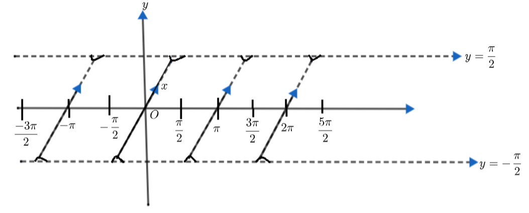
\[{{\sin }^{-1}}\left( \sin x \right)=\left\{ \begin{align} & x;\text{ }-\dfrac{\pi }{2}\le x\le \dfrac{\pi }{2} \\ & \left( \pi -x \right);\text{ }-\dfrac{\pi }{2}\le \pi -x < \dfrac{\pi }{2}\left( \text{i}\text{.e}\text{.,}\dfrac{\pi }{2}\le x\le \dfrac{3\pi }{2} \right) \\ \end{align} \right.\]

\[\Rightarrow {{\sin }^{-1}}\left( \sin x \right)=\left\{ \begin{align} & x,\text{ }-\dfrac{\pi }{2}\le x\le \dfrac{\pi }{2} \\ & \pi -x,\text{ }\dfrac{\pi }{2}\le x\le \dfrac{3\pi }{2}, \\ \end{align} \right.\]

This is plotted as

Thus, we can note that the graph for \[y={{\sin }^{-1}}\left( \sin x \right)\] is a straight line up and a straight line down with slopes \[1\] and \[-1\] respectively lying between \[\left[ -\dfrac{\pi }{2},\dfrac{\pi }{2} \right]\].

The below result for the definition of \[{{\sin }^{-1}}\left( \sin x \right)\] must be kept in mind. \[y={{\sin }^{-1}}\left( \sin x \right)=\left\{ \begin{align} & x+2\pi ;\text{ }-\dfrac{5\pi }{2}\le x\le -\dfrac{3\pi }{2} \\ & -\pi -x;\text{ }-\dfrac{3\pi }{2}\le x\le -\dfrac{\pi }{2} \\ & x;\text{ }-\dfrac{\pi }{2}\le x\le \dfrac{\pi }{2} \\ & \pi -x;\text{ }\dfrac{\pi }{2}\le x\le \dfrac{3\pi }{2} \\ & x-2\pi ;\text{ }\dfrac{3\pi }{2}\le x\le \dfrac{5\pi }{2}\text{ }...\text{and so on} \\ \end{align} \right.\]

Now we consider \[y={{\cos }^{-1}}\left( \cos x \right)\] which is periodic and has period \[2\pi \].

To draw this graph, we should draw the graph for one interval of length \[2\pi \] and repeat the entire values of \[x\] of length \[2\pi \]        

As we know,

\[{{\cos }^{-1}}\left( \cos x \right)=\left\{ \begin{align} & x;\text{ }0\le x\le \pi \\ & 2\pi -x;\text{ }0\le 2\pi -x\le \pi , \\ \end{align} \right.\] \[\Rightarrow {{\cos }^{-1}}\left( \cos x \right)=\left\{ \begin{align} & x;\text{ }0\le x\le \pi \\ & 2\pi -x;\text{ }\pi \le x\le 2\pi , \\ \end{align} \right.\]

Thus, it has been defined for \[0 < x < 2\pi \] that has length \[2\pi \].

So, its graph could be plotted as;

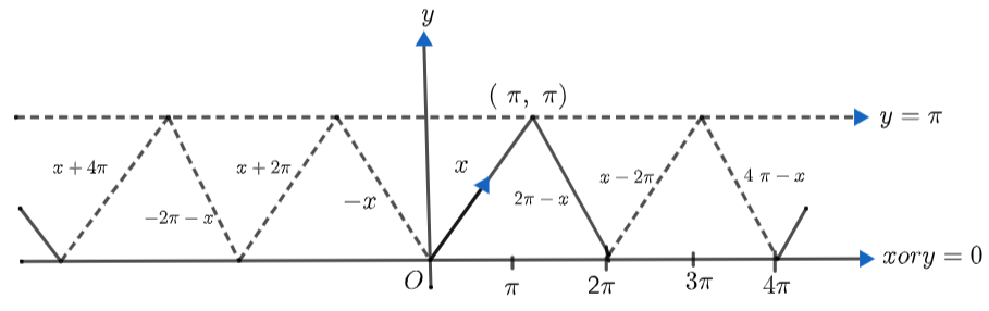
Thus, the curve \[y={{\cos }^{-1}}\left( \cos x \right)\] and we can not the results as \[{{\cos }^{-1}}\left( \cos x \right)=\left\{ \begin{align} & -x,\text{ if x}\in \left[ -\pi ,0 \right] \\ & x,\text{ if x}\in \left[ 0,\pi \right] \\ & 2\pi -x,\text{ if x}\in \left[ \pi ,2\pi \right] \\ & -2\pi +x,\text{ if x}\in \left[ 2\pi ,3\pi \right]\text{ and so on}\text{.} \\ \end{align} \right.\]

Next, we consider \[y={{\tan }^{-1}}\left( \tan x \right)\] which is periodic and has period \[\pi \].

To draw this graph, we should draw the graph for one interval of length \[\pi \] and repeat the entire values of x.

We know \[{{\tan }^{-1}}\left( \tan x \right)=\left\{ x;-\dfrac{\pi }{2} < x < \dfrac{\pi }{2} \right\}\]. Thus, it has been defined for \[-\dfrac{\pi }{2} < x < \dfrac{\pi }{2}\] that has length \[\pi \].

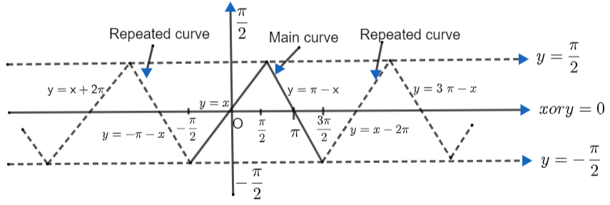
The graph is plotted as

Thus, the curve for \[y={{\tan }^{-1}}\left( \tan x \right)\], where \[y\] is not defined for \[x\in \left( 2n+1 \right)\dfrac{\pi }{2}\]. The below result can be kept in mind.

\[{{\tan }^{-1}}\left( \tan x \right)=\left\{ \begin{align} & -\pi -x,\text{ if x}\in \left[ -\dfrac{3\pi }{2},-\dfrac{\pi }{2} \right] \\ & x,\text{ if x}\in \left[ -\dfrac{\pi }{2},\dfrac{\pi }{2} \right] \\ & x-\pi ,\text{ if x}\in \left[ \dfrac{\pi }{2},\dfrac{3\pi }{2} \right] \\ & x-2\pi ,\text{ if x}\in \left[ \dfrac{3\pi }{2},\dfrac{5\pi }{2} \right]\text{ and so on}\text{.} \\ \end{align} \right.\]

Additional Formulas

1. \[{{\sin }^{-1}}x+{{\sin }^{-1}}y={{\sin }^{-1}}\left( x\sqrt{1-{{y}^{2}}}+y\sqrt{1-{{x}^{2}}} \right)\]

2. \[{{\sin }^{-1}}x-{{\sin }^{-1}}y={{\sin }^{-1}}\left( x\sqrt{1-{{y}^{2}}}-y\sqrt{1-{{x}^{2}}} \right)\]

3. \[{{\cos }^{-1}}x+{{\cos }^{-1}}y={{\cos }^{-1}}\left( xy-\sqrt{1-{{x}^{2}}}\sqrt{1-{{y}^{2}}} \right)\]

4. \[{{\cos }^{-1}}x-{{\cos }^{-1}}y={{\cos }^{-1}}\left( xy+\sqrt{1-{{x}^{2}}}\sqrt{1-{{y}^{2}}} \right)\]

5. \[{{\tan }^{-1}}x+{{\tan }^{-1}}y+{{\tan }^{-1}}z={{\tan }^{-1}}\left[ \dfrac{x+y+z-xyz}{1-xy-yz-zx} \right]\], if \[x>0,y>0,z>0\And xy+yz+zx < 1\]

6. \[{{\tan }^{-1}}x+{{\tan }^{-1}}y+{{\tan }^{-1}}z=\pi \] when \[x+y+z=xyz\]

7. \[{{\tan }^{-1}}x+{{\tan }^{-1}}y+{{\tan }^{-1}}z=\dfrac{\pi }{2}\] when \[xy+yz+zx=1\]

8. \[{{\sin }^{-1}}x+{{\sin }^{-1}}y+{{\sin }^{-1}}z=\dfrac{3\pi }{2}\text{; }x=y=z=1\]

9. \[{{\cos }^{-1}}x+{{\cos }^{-1}}y+{{\cos }^{-1}}z=3\pi ;\text{ }x=y=z=-1\]

10. \[{{\tan }^{-1}}1+{{\tan }^{-1}}2+2{{\tan }^{-1}}3={{\tan }^{-1}}1+{{\tan }^{-1}}\dfrac{1}{2}+{{\tan }^{-1}}\dfrac{1}{3}=\dfrac{\pi }{2}\]

5 Important Formulas for Maths Class 12 Chapter 2 You Shouldn’t Miss!

Importance of Maths Chapter 2 Notes Inverse Trigonometric Functions Class 12

• These notes simplify the understanding of inverse trigonometric functions, which are essential for solving complex maths problems.

• They help students grasp the concept of principal value branches, which is important for accurate calculations.

• The notes clarify the domain and range of inverse trigonometric functions, which is important for solving equations.

• They enhance problem-solving skills by providing clear explanations and examples of how these functions are used in various mathematical contexts.

• Inverse Trigonometric Functions Class 12 Notes PDF aligns with the CBSE Class 12 Maths syllabus, helping students prepare effectively and confidently for board exams.

Tips for Learning the Class 12 Science Chapter 2 Inverse Trigonometric Functions

• Start by thoroughly understanding the basic concepts of trigonometric functions, as this foundation is crucial for grasping inverse trigonometric functions.

• Focus on principal value branches, as they can be challenging; practice identifying them for different functions.

• Ensure you understand the domain and range of each inverse trigonometric function by practising related problems.

• Study the graphs of inverse trigonometric functions to grasp their behaviour and range.

• Practice solving various problems involving inverse trigonometric functions to solidify your understanding and prepare for exams.

Conclusion

The Revision Notes for Class 12 Maths Chapter on Inverse Trigonometric Functions simplify complex ideas, making them easier to grasp. They clearly explain key concepts such as principal value branches, domain, range, and the properties of inverse trigonometric functions. Inverse Trigonometric Functions Class 12 Notes PDF include helpful summaries and practice problems to reinforce learning. This chapter demonstrates how inverse trigonometric functions work and how to solve related problems. Regularly reviewing these notes will help students master the topic and perform better in their Class 12 Maths exams.

Related Study Materials for Class 12 Maths Chapter 2 Inverse Trigonometric Functions

Chapter-wise Revision Notes Links for Class 12 Maths

Important Study Materials for Class 12 Maths