


Maths Notes for Chapter 13 Statistics Class 11 - FREE PDF Download
Section–A (1 Mark Questions)
1. What is the mean deviation of x observations x1,x2,x3,...,xn from their mean.
Ans. $M D=\frac{1}{n} \sum_{i=1}^n\left|x_i-\bar{x}\right|$.
2. If x1,x2,...,xn be n observations and $\bar{x}$ be their arithmetic mean. Then, what is the formula for the standard deviations.
Ans. The formula for $\mathrm{S} . \mathrm{D}=\sigma=\sqrt{\frac{\sum\left(x_i-\bar{x}\right)^2}{n}}$.
3. Coefficient of variation $=\frac{----}{Mean}\times 100$ .
Ans. $C V=\dfrac{S D}{\text { Mean }} \times 100$.
Hence, the value of the filler is SD.
4. If $\bar{x}$ is the mean of n values of x, then $\sum_{i=1}^n\left(x_i-\bar{x}\right)$ is always equal to ..................
Ans. If $\bar{x}$ is the mean of $\mathrm{n}$ observations of $x$, then $\sum_{i=1}^n\left(x_i-\bar{x}\right)=0$ and if ' $a$ ' has the value other than $\bar{x}$, then $\sum_{i=1}^n\left(x_i-\bar{x}\right)^2$ is less then $\sum\left(x_i-a\right)^2$
5. If the variance of a data is 121, then the standard deviations of the data is ..................
Ans. We know that
$$S D=\sqrt{\text { variance }}=\sqrt{121}=11$$
Hence, the value of the filler is 11 .
Section–B (2 Marks Questions)
6. (i) The standard deviation of a data is ................... of any change in origin but is ..................... of change of scale.
(ii) The sum of squares of the deviations of the values of the variable is ................... when taken about their arithmetic mean.
Ans. (i) Since the standard deviation of any data is independent of any change in origin but is dependent of any change of scale.
Hence, the value of the fillers are independent and dependent.
(ii) The sum of the squares of the deviations of the value of variable is minimum when taken about their arithmetic mean. Hence, the value of the filler is minimum.
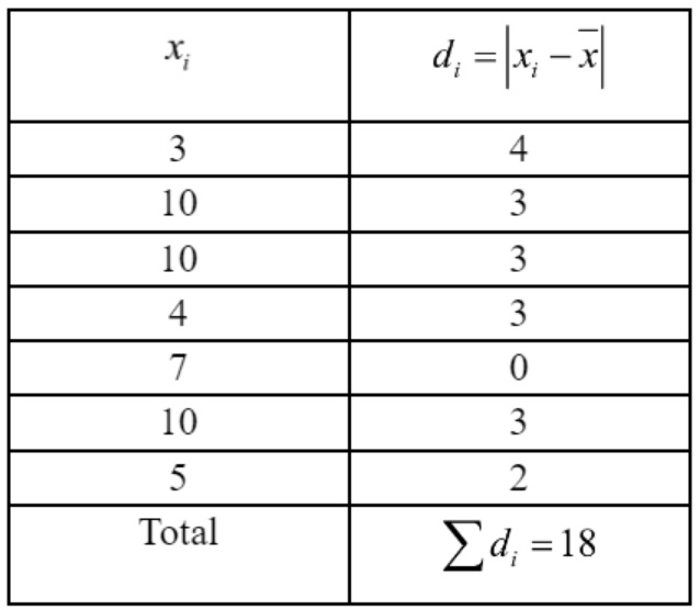
7. Find the mean deviation of the data 3, 10, 10, 4, 7, 10, 5 from the mean.
Ans.
Observations are given by $3,10,10,4,7$, 10 and 5
$$\begin{aligned}& \therefore \bar{x}=\frac{3+10+10+4+7+10+5}{7}=\frac{49}{7}=7 \\& M D=\frac{\sum d_i}{n}=\frac{18}{7}=2.57\end{aligned}$$
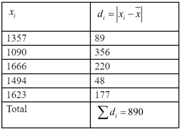
8. The lives (in hours) of 5 bulbs were noted as follows: 1357, 1090, 1666, 1494, 1623. Find the mean deviation (in hours) from their mean.
Ans. he lives of 5 bulbs are given by $1357,1090,1666,1494,1623$
$$\therefore \text { Mean }=\frac{1357+1090+1666+1494+1623}{5}$$
$$\Rightarrow \bar{x}=\frac{7230}{5}=1446$$
$$\therefore E=\frac{\sum d_i}{n}=\frac{890}{5}=178 \text {. }$$
9. If the mean of 100 observations is 50 and their standard deviation is 5, then find the sum of all the squares of all the observation.
Ans. Here $\bar{x}=\frac{\sum x_i}{n}$
$$\begin{aligned}& 50=\frac{\sum x_i}{100} \Rightarrow \sum x_i=5000 \\& \therefore S D=\sqrt{\frac{\sum x_i^2}{n}-\left(\frac{\sum x_i}{n}\right)^2} \\& 5=\sqrt{\frac{\sum x_i^2}{100}-\left(\frac{5000}{100}\right)^2} \Rightarrow25=\frac{\sum x_i^2}{100}-2500 \\& \Rightarrow \frac{\sum x_i^2}{100}=2500+25 \Rightarrow \frac{\sum x_i^2}{100}=2525 \\& \therefore \sum x_i^2=2525 \times 100=252500 .\end{aligned}$$
10. If x1,x2,x3,x4 and x5 be the observations with mean m and standard deviations S then, find the standard deviation of the observations Kx1, Kx2, Kx3, Kx4 and Kx5.
Ans. Here
$$\begin{aligned}& m=\frac{\sum x_i}{N}, S=\sqrt{\frac{\sum x_i^2}{5}-\left(\frac{\sum x_i}{5}\right)^2} \\& \therefore S D=\sqrt{\frac{K^2 \sum x_i^2}{5}-\left(\frac{K \sum x_i}{5}\right)^2} \\& =\sqrt{\frac{K^2 \sum x_i^2}{5}-K^2\left(\frac{\sum x_i}{5}\right)^2} \\& =K \sqrt{\frac{\sum x_i^2}{5}-\left(\frac{\sum x_i}{5}\right)^2} \\& =K \cdot S .\end{aligned}$$
11. Find the standard deviation for first 10 natural numbers as $f(x)=\frac{3x-4}{5}$ then write $f^{-1}(x)$ .
Ans.
$$11. We know that $\mathrm{SD}$ of first $\mathrm{n}$ natural numbers $\sqrt{\frac{n^2-1}{12}}$
Here $n=10$
$$\therefore S D=\sqrt{\frac{(10)^2-1}{12}}=\sqrt{\frac{99}{12}}=\sqrt{8.25}=2.87 \text {.}$$
12. The following information relates to a sample of total frequency 60: $\sum x^{2}=18000$ and $\sum x=960$ then find the variance.
Ans. We know that variance
$$\begin{aligned}& (\sigma)^2=\frac{\sum x_i^2}{N}-\left(\frac{\sum x_i}{N}\right)^2 \\& =\frac{18000}{60}-\left(\frac{960}{60}\right)^2=300-256=44 .\end{aligned}$$
13. The standard deviations of some temperature data in $^{\circ}C$ is 5. If the data were converted into $^{\circ}F$ then what would be the new variance.
Ans. Given that $\sigma_C=5$
We know that
$$\begin{aligned}& C=\frac{5}{9}(F-32) \Rightarrow F=\frac{9 C}{5}+32 \\& \therefore \sigma_F=\frac{9}{5} \sigma_C=\frac{9}{5} \times 5=9 \\& \therefore \sigma_F^2=(9)^2=81 .\end{aligned}$$
PDF Summary - Class 11 Maths Statistics (Chapter 13)Terminologies:
Statistics – It is the science of collection, organization, presentation, analysis and interpretation of the numerical data.
Limit of the class – The end values of a class is called its limits. The highest value is the upper limit and the lowest value is the lower limit.
Class interval – The difference between the upper and lower limit of each class.
Primary and secondary data – The data when collected by the investigator himself is termed as primary data and when it is collected by someone other than the investigator, then it is called the secondary data.
Variable or variate – A symbol or characteristic, whose magnitude varies from observation to observation is called a variable or variate. e.g., weight, height etc.
Frequency – The number of times a given observation occurs in a given set of data is called frequency of that observation.
Discrete frequency distribution – The frequency distribution in which the data is presented in a way that the exact measurements of the units are clearly visible is called a discrete frequency distribution.
Continuous frequency distribution – The frequency distribution in which the classes groups are not exactly measurable is called continuous frequency distribution.
Cumulative frequency distribution – The frequency obtained after adding the frequency of first class to the second class and then to the third class and so on, then the final frequency obtained is called the cumulative frequency. The frequencies given should be in the form of grouped or class frequencies.
Graphical Representation Of Frequency Distribution:
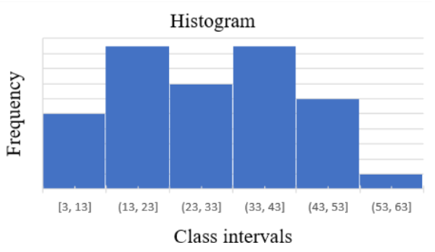
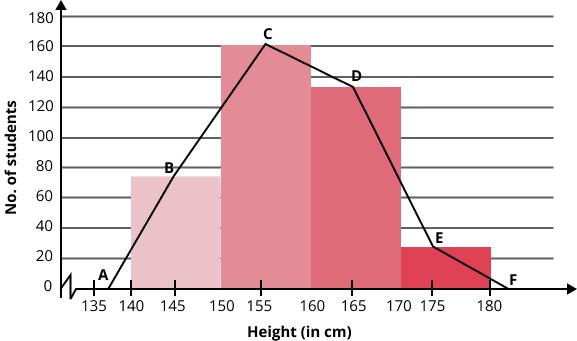
Histogram – A histogram is drawn by marking the given class intervals on x-axis and corresponding frequencies on y-axis. In the corresponding intervals, an erected rectangle is drawn having width proportional to the class interval and length proportional to the frequency of that class interval. When we take the class interval is taken as unit length on the graph, then the frequency of that class denotes the area of the rectangle.
When the class intervals are of unequal widths, then the height of the rectangles are proportional to the ratio of the frequencies to the width of each class. A sample of histogram has been shown below;
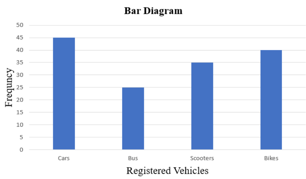
Bar diagram – While drawing bar diagrams, only the length of bars or rectangles are taken into consideration. The data is divided into different classes, then the classes are marked with equal widths on the x-axis and then corresponding frequencies are marked on y-axis which in turn is proportional to the length of each bar. An example has been shown below;
Pie diagrams – These are used to represent relative frequency distribution, in which a circle is divided into sectors which are equal to the number of classes and the area of each sector is proportional to the frequency of that class. The division is done by proportionately dividing the angles as per the frequencies. An example has been shown below;
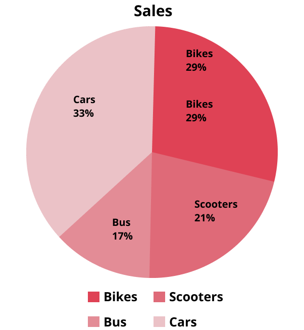
To draw the required sectors, we find the central angles for that which can be calculated using the following relation;
$\text{Central angle}=\dfrac{Frequency\times {{360}^{{}^\circ }}}{\text{Total frequency}}$
Frequency Polygon – In order to draw the frequency polygon of an ungrouped frequency distribution, the variate values are plotted on the x-axis and the corresponding frequencies are plotted on the y-axis. The mid-points of each bar are then joined using straight line to show a trend. An example has been shown below;
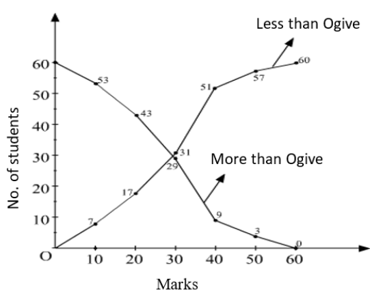
Cumulative frequency curve (Ogive) – We first prepare a cumulative frequency table from the given data. Then we plot the cumulative frequencies against the lower or upper limits of the corresponding class intervals. Then, we join the points and the curve obtained is called a cumulative frequency curve or ogive. Ogives are generally drawn using two methods;
The ‘less than’ method – On the x-axis, plot the points with the upper limits and on the ordinates or y-axis, the corresponding less than cumulative frequencies. Then the points are joined by free hand to het a smooth curve or less than ogive. It is also called a falling curve.
The ‘more than’ method – On the x-axis, plot the points with the lower limits and on the ordinates or y-axis, the corresponding more than cumulative frequencies. Then the points are joined by free hand to het a smooth curve or less than ogive. It is also called a falling curve.
An example has been shown in the diagram below;
Measures Of Central Tendency:
Measures of central tendency is the process of describing a complete data set by using a central value of that data set. The five measures of central tendency are enlisted below:
Arithmetic mean – It is the ratio of the sum of the vales of the items in a series to the total amount of data. These are further of five types;
i) Arithmetic mean for unclassified data – If we have $n$ numbers ${{x}_{1}},{{x}_{2}},{{x}_{3}},....,{{x}_{n}}$, then arithmetic mean is given by;
$A=\overline{X}=\dfrac{{{x}_{1}}+{{x}_{2}}+{{x}_{3}}+....+{{x}_{n}}}{n}$
$=\dfrac{\Sigma _{i=1}^{n}{{x}_{i}}}{n}$.
ii) Arithmetic mean for frequency distribution – If we have $n$ numbers ${{x}_{1}},{{x}_{2}},{{x}_{3}},....,{{x}_{n}}$, such that their corresponding frequencies are ${{f}_{1}},{{f}_{2}},{{f}_{3}},....,{{f}_{n}}$ respectively, then arithmetic mean is given by;
$A=\dfrac{{{f}_{1}}{{x}_{1}}+{{f}_{2}}{{x}_{2}}+{{f}_{3}}{{x}_{3}}+....+{{f}_{n}}{{x}_{n}}}{{{f}_{1}}+{{f}_{2}}+{{f}_{3}}+....+{{f}_{n}}}$
$=\dfrac{\Sigma _{i=1}^{n}{{x}_{i}}{{f}_{i}}}{\Sigma _{i=1}^{n}{{f}_{i}}}$.
iii) Arithmetic mean for classified data – Let us have a class interval with lower limit as $a$ and upper limit as $b$, then the class mark, $x=\dfrac{a+b}{2}$. Now, for a classified data, let the class marks be ${{x}_{1}},{{x}_{2}},{{x}_{3}},....,{{x}_{n}}$ be the variables of the classes, then the arithmetic mean is given by;
\[A=\dfrac{\Sigma xf}{\Sigma f}=\dfrac{\Sigma _{i=1}^{n}\dfrac{1}{2}\left( {{a}_{i}}+{{b}_{i}} \right)\times {{f}_{i}}}{\Sigma _{i=1}^{n}{{f}_{i}}}\].
Step deviation method;
\[A={{A}_{1}}+\left( \dfrac{\Sigma _{i=1}^{n}{{f}_{i}}{{u}_{i}}}{\Sigma _{i=1}^{n}{{f}_{i}}} \right)h\]
Where, ${{A}_{i}}$ is the assumed mean
${{u}_{i}}=\dfrac{{{x}_{i}}-{{A}_{1}}}{h}$
${{f}_{i}}=$frequency
$h=$width of interval
iv) Combined mean – If ${{x}_{1}},{{x}_{2}},{{x}_{3}},....,{{x}_{r}}$ be $r$ groups of observations, then we can find the arithmetic mean of the combined group $x$ using the formula,
$A=\dfrac{{{n}_{1}}{{A}_{1}}+{{n}_{2}}{{A}_{2}}+{{n}_{3}}{{A}_{3}}+....+{{n}_{r}}{{A}_{r}}}{{{n}_{1}}+{{n}_{2}}+{{n}_{3}}+....+{{n}_{r}}}$.
Where,
${{A}_{r}}=$Arithmetic mean of collection ${{x}_{r}}$
${{n}_{r}}=$total frequency of the collection ${{x}_{r}}$
v) Weighted arithmetic mean – The weighted arithmetic mean, if $w$ is the weight of the variable $x$ is given by;
${{A}_{w}}=\dfrac{\Sigma wx}{\Sigma w}$.
Properties Of Arithmetic Mean –
a) Arithmetic means are always independent of change of origin and the change of scale.
b) The algebraic sum of deviations of a set of values with their arithmetic mean is zero.
c) When taken about mean, the sum of the squares of the deviations of a set of values is minimum.
Geometric Mean - If we have $n$ numbers ${{x}_{1}},{{x}_{2}},{{x}_{3}},....,{{x}_{n}}$, then geometric mean is given by;
$G={{\left( \prod\limits_{i=1}^{n}{{{x}_{i}}} \right)}^{\dfrac{1}{n}}}=\sqrt[n]{{{x}_{1}}.{{x}_{2}}.{{x}_{3}}......{{x}_{n}}}$ or
$G=anti\log \left[ \dfrac{\log {{x}_{1}}+\log {{x}_{2}}+...+\log {{x}_{n}}}{n} \right]$
For frequency distribution, we can have
$G={{\left( {{x}_{1}}{{f}_{1}}.{{x}_{2}}{{f}_{2}}.....{{x}_{n}}{{f}_{n}} \right)}^{\dfrac{1}{N}}}$
Where $N=\sum\limits_{i=1}^{n}{{{f}_{i}}}$
Or, $G=anti\log \left[ \dfrac{{{f}_{1}}\log {{x}_{1}}+{{f}_{2}}\log {{x}_{2}}+...+{{f}_{n}}\log {{x}_{n}}}{N} \right]$
Harmonic mean - If we have $n$ numbers ${{x}_{1}},{{x}_{2}},{{x}_{3}},....,{{x}_{n}}$, then harmonic mean is given by;
$HM=\dfrac{n}{\dfrac{1}{{{x}_{1}}}+\dfrac{1}{{{x}_{2}}}+...+\dfrac{1}{{{x}_{n}}}}=\dfrac{n}{\sum\limits_{i=1}^{n}{\dfrac{1}{{{x}_{i}}}}}$
If the corresponding frequencies are ${{f}_{1}},{{f}_{2}},{{f}_{3}},....,{{f}_{n}}$, then
$HM=\dfrac{{{f}_{1}}+{{f}_{2}}+{{f}_{3}}+....+{{f}_{n}}}{\dfrac{{{f}_{1}}}{{{x}_{1}}}+\dfrac{{{f}_{2}}}{{{x}_{2}}}+...+\dfrac{{{f}_{n}}}{{{x}_{n}}}}=\dfrac{\sum\limits_{i=1}^{n}{{{f}_{i}}}}{\sum\limits_{i=1}^{n}{\dfrac{{{f}_{i}}}{{{x}_{i}}}}}$
Median – When we arrange a given set of data in ascending or descending order, then the value lying in the middle is the median of the given data set. It is denoted by ${{M}_{d}}$ and is an average of the position of the numbers.
i) Median for simple distribution – In this type of distribution, first we arrange the terms in either in the ascending order or in the descending order and then find the number of terms $n$.
a) When $n$ is odd, then median is the $\left( \dfrac{n+1}{2} \right)th$ term.
b) When $n$ is even, there will be two terms in the middle. Then the median will be the mean of two middle terms $\dfrac{n}{2}th$ and $\left( \dfrac{n}{2}+1 \right)th$.
ii) Median for unclassified frequency distribution – First, find $\dfrac{N}{2}$, where $N=\Sigma {{f}_{i}}$. Then find the cumulative frequency of the data given and then see the value of the variable which is just greater than or equal to $\dfrac{N}{2}$. This value of the variable is called as the median.
iii) Median of classified data (median class) - First, find $\dfrac{N}{2}$. Then find the cumulative frequency of each class then see the value of the cumulative frequency that is just greater than or equal to $\dfrac{N}{2}$. The corresponding class is the median class.
For a continuous distribution, median is given by
${{M}_{d}}=l+\left( \dfrac{\dfrac{N}{2}-C}{f} \right)\times h$
Where, $l=$lower limit of the median class
$f=$frequency of the median class
$N=\sum{f}$=total frequency
$C=$cumulative frequency of the class preceding the median class
$h=$length of the median class
Quartiles – Like median, a distribution can also be divided into more equal parts (four, five, six etc.). The quartiles for a continuous distribution are given by
${{Q}_{1}}=l+\left( \dfrac{\dfrac{N}{4}-C}{f} \right)\times h$.
Where, $l=$lower limit of the quartile class
$f=$frequency of the quartile class
$N=$$\Sigma f$=total frequency
$C=$cumulative frequency of the class preceding the first quartile class
$h=$length of the quartile class
Similarly,
${{Q}_{3}}=l+\left( \dfrac{\dfrac{3N}{4}-C}{f} \right)\times h$.
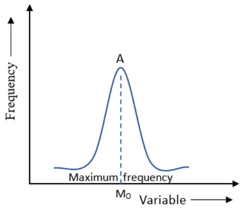
Mode – The value at the point about which the data set tend to be most highly concentrated is called the mode ${{M}_{o}}$ of the distribution.
i) Mode for a raw data – Suppose we have the following numbers of a variable $70,80,90,96,70,96,96,90$, then the mode will be $96$ as it occurs maximum number of times. Graphically mode can be represented as follows;
ii) For classified distribution – In case of datasets divided into classes then the class with maximum frequency is called the modal class and the middle point of that modal class is called is called the crude mode. The class preceding and succeeding the modal class are called the pre-modal and post-modal class respectively.
iii) Mode for classified data (continuous distribution) – The mode is given by;
${{M}_{O}}=l+\left( \dfrac{{{f}_{0}}-{{f}_{1}}}{2{{f}_{0}}-{{f}_{1}}-{{f}_{2}}} \right)\times h$
Where, $l=$ lower limit of modal class
${{f}_{0}}=$ frequency of the modal class
${{f}_{1}}=$ frequency of the pre-modal class
${{f}_{2}}=$ frequency of the post-modal class
$h=$ length of class interval
Relation between mean, Median and Mode –
i) $Mean-Mode=3\left( Mean-Median \right)$
ii) $Mode=3Median-2Mean$
Symmetrical And Skew Distribution:
A distribution is said to be symmetric if same number of frequencies is distributed on either side of the mode. In this case the frequency curve is bell-shaped and $A={{M}_{d}}={{M}_{o}}$.

The variation does not have symmetry in the case of an anti-symmetric or skew distribution. Considering two cases,
(i) Positive skewness - The frequencies increases sharply in the beginning and decreases slowly after the modal value and $A > {{M}_{d}} > {{M}_{o}}$.

(ii) Negative skewness - The frequencies increases slowly in the beginning and decreases slowly after the modal value and $A < {{M}_{d}} < {{M}_{o}}$.

Measure Of Dispersion:
Dispersion of the data is the degree to which numerical data tend to spread about an average value. There are three dispersions, enlisted below:
Range is used to denote the difference between the highest and the lowest element of a data. It can be represented as $range={{x}_{\max }}-{{x}_{\min }}$.
The coefficient of range is expressed as $\dfrac{{{x}_{\max }}-{{x}_{\min }}}{{{x}_{\max }}+{{x}_{\min }}}$.
It finds its uses in statists, especially in series relating to quality control in production.
i) Inter-quartile range is ${{Q}_{3}}-{{Q}_{1}}$.
ii) Semi-inter quartile range (quartile deviation) is QD = $\dfrac{{{Q}_{3}}-{{Q}_{1}}}{2}$
iii) Coefficient of quartile deviation is $\dfrac{{{Q}_{3}}-{{Q}_{1}}}{{{Q}_{3}}+{{Q}_{1}}}$
iv) \[QD=\dfrac{2}{3}SD\]
Mean Deviation is defined as the arithmetic mean of absolute deviations of the values of the variable from a measure of their average, which can be either of mean, median, or mode. $\delta $ is used to denote it. The formula for various conditions is below,
i) For simple (discrete) distribution $\delta =\sum{\dfrac{\left| x-z \right|}{n}}$, where n is the number of terms and z can be either of A or ${{M}_{d}}$ or ${{M}_{o}}$.
ii) For unclassified frequency distribution $\delta =\dfrac{\sum \left| x-z \right|}{\sum f}$
iii) For classified distribution $\delta =\dfrac{\sum \left| x-z \right|}{\sum f}$, x is for class mark of the interval.
iv) $MD=\dfrac{4}{5}SD$
v) Average (mean or Median or Mode) $=\dfrac{mean\text{ }deviation\text{ }from\text{ }the\text{ }avergae}{average}$
vi) Coefficient of Mean Deviation is the ratio of MD and the mean from which the deviation is measured and is given by $MD=\dfrac{\sum \left| x-\overline{x} \right|}{n}$.
Standard deviation is defined as the square root of the arithmetic mean of the squares of deviations of the terms from their arithmetic mean. It is denoted by $\sigma $. The formulas are as below,
i) For simple distribution $\sigma =\sqrt{\dfrac{\sum {{\left( x-\overline{x} \right)}^{2}}}{n}}=\sqrt{\dfrac{\sum {{d}^{2}}}{n}}$.
ii) For frequency distribution $\sigma =\sqrt{\dfrac{\sum f{{\left( x-\overline{x} \right)}^{2}}}{\sum f}}=\sqrt{\dfrac{\sum f{{d}^{2}}}{\sum f}}$.
iii) For classified data $\sigma =\sqrt{\dfrac{\sum f{{\left( x-\overline{x} \right)}^{2}}}{\sum f}}=\sqrt{\dfrac{\sum f{{d}^{2}}}{\sum f}}$ x is the class mark.
iv) Shortcut Method for SD $\sigma =\sqrt{\dfrac{\sum f{{d}^{2}}}{\sum f}-{{\left( \dfrac{\sum fd}{\sum f} \right)}^{2}}}$, where \[d=x-A'\] and $A'$ is the assumed mean.
v) Standard deviation of the Combined Series – If ${{n}_{1}},{{n}_{2}}$ are the sizes, $\overline{{{X}_{1}}},\overline{{{X}_{2}}}$ are the means and ${{\sigma }_{1}},{{\sigma }_{2}}$ are the standard deviation of the series, then the standard deviation of the combined series is given by $\sigma =\sqrt{\dfrac{{{n}_{1}}\left( {{\sigma }_{1}}^{2}+{{d}_{1}}^{2} \right)+{{n}_{2}}\left( {{\sigma }_{2}}^{2}+{{d}_{2}}^{2} \right)}{{{n}_{1}}+{{n}_{2}}}}$ , where ${{d}_{1}}=\overline{{{X}_{1}}}-\overline{X}\text{ }and\text{ }{{d}_{2}}=\overline{{{X}_{2}}}-\overline{X}$
Variance is the square of standard deviation and ${{\sigma }^{2}}$ is used to denote it.
Analysis of Frequency Distributions:
The measure of variability is called as the coefficient of variation. It is independent of units. The letters C.V. is used for denoting it. It is defined as $C.V=\dfrac{\sigma }{\overline{x}}\times 100$, where the term $\dfrac{\sigma }{\overline{x}}$ is called coefficient of standard deviation.
The distribution for which the coefficient of variation is less is called more consistent.
For two series with equal means, the series with greater standard deviation is called more variable than the other.
The series with lesser value of standard deviation is said to be more consistent than the other.
Notes of Statistics Class 11 Statistics – Brief Chapter Overview
Class 11 Maths Revision Notes Chapter 13 PDF
With the entire Class 11 Revision Notes Statistics available in PDF format on the official website of Vedantu, you have your mathematics revision at your fingertips. Download and save them on your device or print them out in a hard copy for a quick revision of all important formulas anytime, anywhere, even on the go without an internet connection. The Class 11 Statistics Notes are made keeping in mind the understanding level of class 11 students; hence you will be able to grasp all the problems discussed easily.
Revision Notes Class 11 Maths Chapter 13
Definition of Statistics and some Useful Terms - Statistics is used to collect, organize, and present numerical data for its analysis and interpretation. Some important terms associated with statistics are:
Limit of the Class - In a class, the smallest and the largest data values that can go in it are called the limit of the class.
Class Interval - It is also called the size of the class and is measured as the difference between the upper and lower limit of the class.
Primary and Secondary Data - The data which the investigator himself/herself collects is called the primary data. The data which others (not the investigator) collect is termed as secondary data.
Variable or Variate - Any parameter of the data whose magnitude changes from one observation to another is a variable. Examples of variates are age, weight, height, etc.
Frequency - The frequency of a given observation is the number of times it occurs in the data.
Discrete Frequency Distribution - If the exact measurements of units are clearly shown in the data presented, then that frequency distribution is termed as Discrete Frequency Distribution.
Continuous Frequency Distribution - If the exact measurements of units are not clear and data are presented as classes or groups, then that frequency distribution is termed as Continuous Frequency Distribution.
Graphical Representation of Frequency Distribution
Histogram - To draw a histogram, all the class intervals are marked on the x-axis. Then vertical rectangles are erected on each interval. The height of these rectangles is proportional to the frequency distribution of that class group, and the area enclosed within each rectangle represents the frequency distribution of that class interval.
Bar Diagram - Bar diagrams are drawn by marking equal lengths on the x-axis for different classes. Only the bars' lengths are taken into consideration, which is proportional to the frequency distribution of that class.
Pie Diagrams - Pie diagrams are based on the relative frequency distribution. In a pie diagram, we draw a circle and then divide it into as numerous sectors as there are classes in a frequency distribution. The relative frequency of a class determines the area and angle of each sector.
Frequency Polygon - This is used to represent an ungrouped frequency distribution. Points are plotted whose abscissae is the variate value and ordinates are the frequencies. Then we join these points by a straight line to get the frequency polygon.
Arithmetic Mean - The arithmetic mean is calculated by summing the group of numbers and dividing it by the number of groups. It is denoted as:
For unclassified data, if there are n numbers as a1, a2, a3, …,an then it's AM = \[\overline{A}\] = (\[\sum_{i=1}^{n}\]ai)/n
If frequency distributions are known and f1, f2, f3, …, fn are the frequencies corresponding to a1, a2, a3, ...an then A = (\[\sum_{i=1}^{n}\]aifi)/\[\sum_{i=1}^{n}\]fi
For classified data, the class marks are taken as variables, and AM is defined as A = (\[\sum_{i=1}^{n}\]½ (xi + yi) * fi)/\[\sum_{i=1}^{n}\]fi. Here the class mark of the class interval is (x - y).
FAQs on CBSE Notes Class 11 Maths Chapter 13 - Statistics - 2026-27
1. What are the key terms and definitions students must understand for effective revision of Class 11 Statistics Chapter 13?
Some key terms essential for quick revision of Statistics in Class 11 include:
- Statistics: The science of collecting, organizing, presenting, analyzing, and interpreting numerical data.
- Class Interval: The difference between upper and lower class limits in a frequency distribution.
- Primary Data & Secondary Data: Primary is collected by the investigator; secondary is collected by someone else.
- Frequency: The number of times an observation occurs in a dataset.
- Mean, Median, Mode: Measures of central tendency that summarize data with a single representative value.
2. How can students structure their chapter-wise revision for Statistics in Class 11 according to the CBSE 2026–27 syllabus?
To revise Statistics Class 11 efficiently as per the current CBSE syllabus, students should:
- Start with understanding core definitions and terms (e.g., mean, median, mode, frequency distributions).
- Quickly review summary tables or concept maps for formulas and graphical methods.
- Practice basic calculations for central tendency and dispersion (mean deviation, standard deviation, variance).
- Interpret and compare different graphical representations (histogram, bar diagram, pie diagram, frequency polygon).
- Recap properties and relationships between measures (e.g., relation between mean, median, mode).
3. What are the main types of frequency distributions and how do they differ?
Frequency distributions in Class 11 Statistics include:
- Discrete frequency distribution: Shows distinct, separate values and their frequencies.
- Continuous frequency distribution: Groups data into intervals, not showing the exact measurements.
- Cumulative frequency distribution: Summarizes frequencies cumulatively across intervals.
The main difference is how data values are presented—discrete for separate values, continuous for interval-based grouping.
4. What is the importance of graphical representation in Statistics revision notes and which types should students master?
Graphical representation is crucial because it helps visualize data trends and frequency distributions quickly for revision. Students should master:
- Histogram – For continuous data.
- Bar diagram – For comparison between discrete categories.
- Pie diagram – For proportions and relative frequency.
- Frequency polygon – For ungrouped distributions.
- Ogive (Cumulative frequency curve) – For understanding cumulative frequencies.
5. How do measures of central tendency (mean, median, mode) help summarise data in Statistics Class 11?
Measures of central tendency like mean, median, and mode provide a single value that describes the center or typical value of a dataset. They simplify complex data and help in quick decision making during revision. Each measure is suitable for different types of data and distributions.
6. What are the different methods to calculate arithmetic mean for various data types found in CBSE Class 11 Statistics?
Arithmetic mean can be calculated using several methods:
- For unclassified data: Add all values and divide by total number of values.
- For frequency distribution: Multiply each value by its frequency, sum these, then divide by total frequency.
- For classified data: Use class marks and frequencies to find the mean.
- Step deviation and assumed mean methods can simplify calculations for large or grouped data.
7. What is mean deviation in Statistics and how does it differ from standard deviation?
Mean deviation is the average of the absolute differences between data points and a central value (mean, median, or mode). Standard deviation measures how much values deviate from the mean using squares of differences, making it more sensitive to outliers. Both quantify dispersion, but standard deviation is more widely used and has key formula properties.
8. How can understanding properties of measures like mean and variance prevent common mistakes during revision?
Knowing the properties helps avoid misconceptions, such as:
- The sum of deviations from mean is always zero.
- Variance is always non-negative and is minimized when deviations are measured from the mean.
- Arithmetic mean is independent of change of origin, but dependent on change of scale.
Understanding these prevents calculation errors and helps in verifying answers quickly.
9. Why is it important to distinguish between primary and secondary data when revising Statistics notes?
Distinguishing between primary and secondary data clarifies the source and reliability of data. Primary data is first-hand and usually more reliable for analyses, while secondary data may already be summarized or altered. This awareness improves data interpretation during quick revision and applications in exam questions.
10. How can students revise formulas and properties efficiently before CBSE exams for Statistics Class 11 Chapter 13?
Students should create summary sheets or concept maps of all core formulas, such as those for mean, median, mode, standard deviation, and variance. Practice applying each formula to examples. Use mnemonic aids, flashcards, or teach-back methods to reinforce retention. Regular short revisions just before exams are also recommended for quick recall.
11. What are some application-based questions students should prepare to answer after revising Statistics Class 11 notes?
After revision, students should be able to:
- Calculate the mean, median, and mode for real datasets or exam samples.
- Interpret and draw different graphs based on given data.
- Compare data distributions using standard deviation and variance concepts.
- Identify the type of frequency distribution in practical cases.
- Analyze the significance and consistency of different datasets.