Continuity and Differentiability Class 12 Notes: CBSE Maths Chapter 5

Continuity

1. Definition:

A function $f({\text{x}})$ is said to be continuous at ${\text{x}} = {\text{a}}$; where ${\text{a}} \in $ domain of $f({\text{x}})$, if

$\mathop {\lim }\limits_{x \to {a^ - }} f(x) = \mathop {\lim }\limits_{x \to {a^ + }} f(x) = f(a)$

i.e., ${\text{LHL}} = {\text{RHL}} = $ value of a function at ${\text{x}} = {\text{a}}$

or $\quad \mathop {\lim }\limits_{x \to a} f(x) = f(a)$

1.1 Reasons of discontinuity

If $f({\text{x}})$ is not continuous at ${\text{x}} = {\text{a}}$, we say that $f({\text{x}})$ is discontinuous at $x = a$

There are following possibilities of discontinuity:

1. $\mathop {\lim }\limits_{x \to {a^ - }} f(x)$ and $\mathop {\lim }\limits_{x \to {a^ + }} f(x)$ exist but they are not equal.

2. $\mathop {\lim }\limits_{x \to {a^ - }} f(x)$ and $\mathop {\lim }\limits_{x \to {a^ + }} f(x)$ exists and are equal but not equal to $f(a)$

3. $f(a)$ is not defined.

4. At least one of the limits does not exist. The graph of the function will show a break at the location of discontinuity from a geometric standpoint.

The graph as shown is discontinuous at $x = 1,2$ and 3 .

2. Properties of Continuous Functions 

Let $f({\text{x}})$ and $g({\text{x}})$ be continuous functions at ${\text{x}} = {\text{a}}$. Then,

1. $\quad {\text{c}}f({\text{x}})$ is continuous at ${\text{x}} = {\text{a}}$, where ${\text{c}}$ is any constant.

2. $f({\text{x}}) \pm g({\text{x}})$ is continuous at ${\text{x}} = {\text{a}}$.

3. $f(x) \cdot g(x)$ is continuous at $x = a$.

4. $\quad f({\text{x}})/{\text{g}}({\text{x}})$ is continuous at ${\text{x}} = {\text{a}}$, provided $g({\text{a}}) \ne 0$.-

5. Assuming $f({\text{x}})$ be continuous on $[{\text{a}},{\text{b}}]$ in such a way that the function $f({\text{a}})$ and $f(\;{\text{b}})$ will be at opposite signs, then there will exists at least one solution of equation $f(x) = 0$ in the open interval $(a,b)$

3. The Intermediate Value Theorem 

Suppose $f({\text{x}})$ is continuous on an interval I, also a and b are any two points of $I$. Then if ${y_0}$ is a number between $f(a)$ and $f(b)$, their exits a number $c$ between $a$ and $b$ such that $f(c) = {y_0}$

The Function $f$, being continuous on $(a,b)$ takes on every value between $f(a)$ and $f(b)$

Note:

That a function $f$ which is continuous in [a, b] possesses the following properties:

(i) If $f(a)$ and $f(b)$ possess opposite signs, then there exists at least one solution of the equation $f(x) = 0$ in the open interval $(a,b)$

(ii) If $K$ is any real number between $f(a)$ and $f(b)$, then there exists at least one solution of the equation $f$ $({\text{x}}) = {\text{K}}$ in the open interval $({\text{a}},{\text{b}})$

4. Continuity In An Interval 

(a) A function $f$ is said to be continuous in (a, b) if $f$ is continuous at each and every point $ \in ({\text{a}},{\text{b}})$

(b) A function $f$ is said to be continuous in a closed interval $[{\text{a}},{\text{b}}]$ if :

(1) $f$ is continuous in the open interval $(a,b)$ and

(2) $f$ is right continuous at 'a' i.e. ${\operatorname{Limit} _{x \to {a^ + }}}$ $f({\text{x}}) = f({\text{a}}) = {\text{a}}$ finite quantity

(3) $f$ is left continuous at 'b'; i.e. $\mathop {{\text{Limit }}}\limits_{x \to {b^ - }} $ $f(x) = f(b) = a$ finite quantity

5. A List of Continuous Functions 

6. Types Of Discontinuities 

Type-1 : (Removable type of discontinuities) 

In this case, $\mathop {{\text{Limit}}}\limits_{x \to c} f({\text{x}})$ exists but it will not equal to $f({\text{c}})$ . As a result, the function is said to have a removable discontinuity or discontinuity of the first kind. In such scenario, we can redefine the function such that $\mathop {\operatorname{Limit} }\limits_{x \to c} f(x) = f(c)$ and make it continuous at ${\text{x}} = {\text{c}}$. It can be further categorised as:

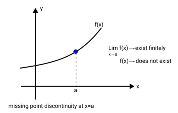
(a) Missing Point Discontinuity:

Where $\mathop {Limit}\limits_{x \to a} f(x)$ exists finitely but $f(a)$ is not defined.

E.g. $f(x) = \dfrac{{(1 - x)\left( {9 - {x^2}} \right)}}{{(1 - x)}}$ will have a missing point discontinuity at $x = 1$, and

$f({\text{x}}) = \dfrac{{\sin {\text{x}}}}{{\text{x}}}$ will have a missing point discontinuity at ${\text{x}} = 0$

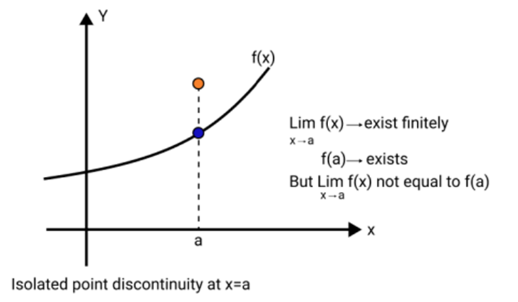
(b) Isolated Point Discontinuity :

Where $\mathop {\operatorname{Limit} }\limits_{x \to a} f(x)$ exists $f$ (a) also exists but;

${\operatorname{Limit} _{{\text{x}} \to {\text{a}}}} \ne f({\text{a}})$

E.g. $f(x) = \dfrac{{{x^2} - 16}}{{x - 4}},x \ne 4$ and $f(4) = 9$ will have an isolated point discontinuity at $x = 4$

In the same way \[f(x) = [x] + [ - x] = \left[ {\begin{array}{*{20}{c}} 0&{{\text{ if }}x \in I} \\ { - 1}&{{\text{ if }}x \notin I} \end{array}} \right] will have an isolated point discontinuity at all x \in I\].

will have an isolated point discontinuity at all x ∈ I.

Type-2 : (Non-Removable type of discontinuities)

In case, $\mathop {\operatorname{Limit} }\limits_{x \to a} f(x)$ does not exist, then it is not possible to make the function continuous by redefining it. Such discontinuities are known as non-removable discontinuity or discontinuity of the 2nd kind. Non-removable type of discontinuity can be further classified as:

(a) Finite Discontinuity:

E.g., $f(x) = x - [x]$ at all integral $x;f(x) = {\tan ^{ - 1}}\dfrac{1}{x}$ at $x = 0$ and $f({\text{x}}) = \dfrac{1}{{1 + {2^{\dfrac{1}{{\text{x}}}}}}}$ at ${\text{x}} = 0$ (note that $\left. {f\left( {{0^ + }} \right) = 0;f\left( {{0^ - }} \right) = 1} \right)$ $1 + {2^ - }$

(b) Infinite Discontinuity:

${\text{ E}}{\text{.g}}{\text{., }}f(x) = \dfrac{1}{{x - 4}}{\text{ or }}g(x) = \dfrac{1}{{{{(x - 4)}^2}}}{\text{ at }}x = 4;f(x) = {2^{\tan x}}$

at $x = \dfrac{\pi }{2}$ and $f(x) = \dfrac{{\cos x}}{x}$ at $x = 0$

(c) Oscillatory Discontinuity:

${\text{ E}}{\text{.g}}{\text{., }}f(x) = \sin \dfrac{1}{x}{\text{ at }}x = 0$

In all these cases the value of $f(a)$ of the function at $x = a$ (point of discontinuity) may or may not exist but $\mathop {{\text{ Limit does }}}\limits_{x \to a} $ not exist.

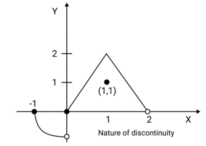
From the adjacent graph note that

$  f $ is continuous at $x =  - 1$

$ f $ has isolated discontinuity at ${\text{x}} = 1$

$ f $ has missing point discontinuity at $x = 2$

$ f $ has non-removable (finite type) discontinuity at the origin.

Note:

(a) In case of dis-continuity of the second kind the nonnegative difference between the value of the RHL at ${\text{x}} = {\text{a}}$ and ${\text{LHL}}$ at ${\text{x}} = {\text{a}}$ is called the jump of discontinuity. A function having a finite number of jumps in a given interval I is called a piece wise continuous or sectionally continuous function in this interval.

(b) All Polynomials, Trigonometrical functions, exponential and Logarithmic functions are continuous in their domains.

(c) If $f({\text{x}})$ is continuous and $g({\text{x}})$ is discontinuous at ${\text{x}} = {\text{a}}$ then the product function $\phi (x) = f(x) \cdot g(x)$ is not necessarily be discontinuous at $x = a$. e.g.

\[f(x) = x{\text{ and }}g(x) = \left[ {\begin{array}{*{20}{c}} {\sin \dfrac{\pi }{x}}&{x \ne 0} \\ 0&{x = 0} \end{array}} \right.\]

(d) If $f({\text{x}})$ and $g({\text{x}})$ both are discontinuous at ${\text{x}} = {\text{a}}$ then the product function $\phi (x) = f(x) \cdot g(x)$ is not necessarily be discontinuous at ${\text{x}} = {\text{a}}.$ e.g

\[f(x) =  - g(x) = \left[ {\begin{array}{*{20}{c}} 1&{x \geqslant 0} \\ { - 1}&{x < 0} \end{array}} \right.\]

(e) Point functions are to be treated as discontinuous 

eg.$f(x) = \sqrt {1 - x}  + \sqrt {x - 1} $ is not continuous at $x = 1$

(f) A continuous function whose domain is closed must have a range also in the closed interval.

(g) If $f$ is continuous at $x = a$ and $g$ is continuous at ${\text{x}} = f$ (a) then the composite $g[f({\text{x}})]$ is continous at ${\text{x}} = {\text{a}}$ 

E.g $f({\text{x}}) = \dfrac{{{\text{x}}\sin {\text{x}}}}{{{{\text{x}}^2} + 2}}$ and $g({\text{x}}) = |{\text{x}}|$ are continuous at ${\text{x}}$ $ = 0$, hence the composite$(gof)({\text{x}}) = \left| {\dfrac{{{\text{x}}\sin {\text{x}}}}{{{{\text{x}}^2} + 2}}} \right|$ will also be continuous at ${\text{x}} = 0$.

Differentiability

1. Definition 

Let $f({\text{x}})$ be a real valued function defined on an open interval $(a,b)$ where $c \in (a,b)$. Then $f(x)$ is said to be differentiable or derivable at $x = c$

if, $\mathop {\lim }\limits_{{\text{x}} \to {\text{c}}} \dfrac{{f({\text{x}}) - f({\text{c}})}}{{({\text{x}} - {\text{c}})}}$ exists finitely.

This limit is called the derivative or differentiable coefficient of the function $f(x)$ at $x = c$, and is denoted by ${f^\prime }({\text{c}})$ or $\dfrac{{\text{d}}}{{{\text{dx}}}}{(f({\text{x}}))_{{\text{x}} = {\text{c}}}}$

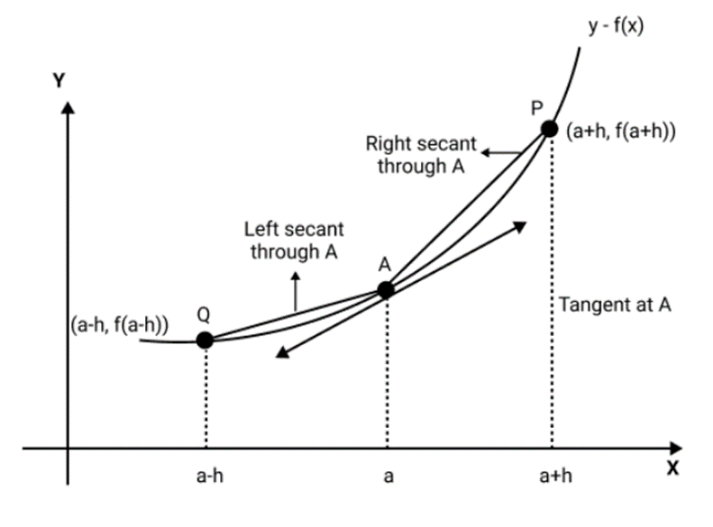
- Slope of Right hand secant $ = \dfrac{{f({\text{a}} + {\text{h}}) - f({\text{a}})}}{{\text{h}}}$ as ${\text{h}} \to 0,{\text{P}} \to {\text{A}}$ and secant $({\text{AP}}) \to $ tangent at ${\text{A}}$

$ \Rightarrow \quad {\text{ Right hand derivative }} = {\operatorname{Lim} _{{\text{h}} \to 0}}\left( {\dfrac{{f({\text{a}} + {\text{h}}) - f({\text{a}})}}{{\text{h}}}} \right)$

$ = \quad $ Slope of tangent at ${\text{A}}$ (when approached from right) ${f^\prime }\left( {{{\text{a}}^ + }} \right)$

- Slope of Left hand secant $ = \dfrac{{f({\text{a}} - {\text{h}}) - f({\text{a}})}}{{ - {\text{h}}}}$ as h $ \to 0,{\text{Q}} \to {\text{A}}$ and secant ${\text{AQ}} \to $ tangent at ${\text{A}}$

$ \Rightarrow \quad {\text{ Left hand derivative }} = {\operatorname{Lim} _{h \to 0}}\left( {\dfrac{{f(a - h) - f(a)}}{{ - h}}} \right)$

= Slope of tangent at ${\text{A}}$ (when approached from left) ${f^\prime }\left( {{{\text{a}}^ - }} \right)$

Thus, $f({\text{x}})$ is differentiable at ${\text{x}} = {\text{c}}$.

\[\begin{array}{*{20}{l}} { \Leftrightarrow \quad \mathop {\lim }\limits_{ \to c} \dfrac{{f() - f({\text{c}})}}{{( - {\text{c}})}}{\text{ exists finitely }}} \\ { \Leftrightarrow \quad \mathop {\lim }\limits_{ \to {{\text{c}}^ - }} \dfrac{{f() - f({\text{c}})}}{{( - {\text{c}})}} = \mathop {\lim }\limits_{ \to {{\text{c}}^ + }} \dfrac{{f() - f({\text{c}})}}{{( - {\text{c}})}}} \\ { \Leftrightarrow \quad \mathop {\lim }\limits_{{\text{h}} \to 0} \dfrac{{f({\text{c}} - {\text{h}}) - f({\text{c}})}}{{ - {\text{h}}}} = \mathop {\lim }\limits_{{\text{h}} \to 0} \dfrac{{f({\text{c}} + {\text{h}}) - f({\text{c}})}}{{\text{h}}}} \end{array}\]

Hence, $\quad \mathop {\lim }\limits_{x \to {c^ - }} \dfrac{{f({\mathbf{x}}) - f({\mathbf{c}})}}{{({\mathbf{x}} - {\mathbf{c}})}} = \mathop {\lim }\limits_{{\mathbf{h}} \to 0} \dfrac{{f({\mathbf{c}} - {\mathbf{h}}) - {\mathbf{f}}({\mathbf{c}})}}{{ - {\mathbf{h}}}}$ is called the left hand derivative of $f(x)$ at $x = c$ and is denoted by ${f^\prime }\left( {{{\text{c}}^ - }} \right)$or ${\text{L}}{f^\prime }({\text{c}})$ While, $\mathop {\lim }\limits_{{\mathbf{x}} \to {{\text{c}}^ + }} \dfrac{{{\mathbf{f}}({\mathbf{x}}) - {\mathbf{f}}({\mathbf{c}})}}{{{\mathbf{x}} - {\mathbf{c}}}} = \mathop {\lim }\limits_{{\mathbf{h}} \to 0} \dfrac{{{\mathbf{f}}({\mathbf{c}} + {\mathbf{h}}) - {\mathbf{f}}({\mathbf{c}})}}{{\mathbf{h}}}$ is called the right hand derivative of $f(x)$ at $x = c$ and is denoted by ${f^\prime }\left( {{{\text{c}}^ + }} \right)$or ${\text{R}}{f^\prime }({\text{c}})$

If ${f^\prime }\left( {{{\text{c}}^ - }} \right) \ne {f^\prime }\left( {{{\text{c}}^ + }} \right)$, we say that $f({\text{x}})$ is not differentiable at $x = c$.

2. Differentiability in a Set 

1. A function $f(x)$ defined on an open interval $(a,b)$ is said to be differentiable or derivable in open interval $(a,b)$, if it is differentiable at each point of $(a,b)$

2. A function $f(x)$ defined on closed interval [a, b] is said to be differentiable or derivable. "If ${\text{f}}$ is derivable in the open interval (a, b) and also the end points a and b, then $f$ is said to be derivable in the closed interval [a, b]"

i.e., $\mathop {\lim }\limits_{ \to {a^ + }} \dfrac{{f() - f(a)}}{{ - a}}$ and $\mathop {\lim }\limits_{ \to {b^ - }} \dfrac{{f() - f(b)}}{{ - b}}$, both exist.

A function $f$ is said to be a differentiable function if it is differentiable at every point of its domain.

Note:

1. If $f(x)$ and $g(x)$ are derivable at $x = $ a then the functions $f(x) + g(x),f(x) - g(x),f(x) \cdot g(x)$ will also be derivable at $x = a$ and if $g(a) \ne 0$ then the function $f({\text{x}})/{\text{g}}({\text{x}})$ will also be derivable at $x = a$

2. If $f(x)$ is differentiable at $x = a$ and $g(x)$ is not differentiable at ${\text{x}} = {\text{a}}$, then the product function ${\text{F}}({\text{x}}) = f({\text{x}}) \cdot g({\text{x}})$ can still be differentiable at ${\text{x}} = {\text{a}}.$ E.g. $f({\text{x}}) = {\text{x}}$ and $g({\text{x}}) = |{\text{x}}|$

3. If $f(x)$ and $g$ (x) both are not differentiable at ${\text{x}} = {\text{a}}$ then the product function; $F({\text{x}}) = f({\text{x}}) \cdot g({\text{x}})$ can still be differentiable at $x = $ a. E.g. $f({\text{x}}) = |{\text{x}}|$ and ${\text{g}}({\text{x}}) = |{\text{x}}|$

4. If $f(x)$ and $g(x)$ both are not differentiable at ${\text{x}} = {\text{a}}$ then the sum function $F({\text{x}}) = f({\text{x}}) + g({\text{x}})$ may be a differentiable function. E.g., $f(x) = |x|$ and $g({\text{x}}) =  - |{\text{x}}|$

5. If $f(x)$ is derivable at $x = a$

$ \Rightarrow {f^\prime }(x)$ is continuous at $x = a$.

e.g. 

\[f(x) = \left[ {\begin{array}{*{20}{c}} 2&{{\text{ if }} \ne 0} \\ 0&{{\text{ if }} = 0} \end{array}} \right.\]

3. Relation Between Continuity and Differentiability

We learned in the last section that if a function is differentiable at a point, it must also be continuous at that point, and therefore a discontinuous function cannot be differentiable. The following theorem establishes this fact.

Theorem: If a function is differentiable at a given point, it must be continuous at that same point. However, the inverse is not always true.

or $\quad f(x)$ is differentiable at $x = c$

$ \Rightarrow \quad f({\text{x}})$ is continuous at ${\text{x}} = {\text{c}}$

Converse: The reverse of the preceding theorem is not always true, i.e., a function might be continuous but not differentiable at a given point.

E.g., The function $f(x) = |x|$ is continuous at $x = 0$ but it is not differentiable at ${\text{x}} = 0$.

Note:

(a) Let ${f^{\prime  + }}(a) = p;\,{f^{\prime  - }}(a) = q$ where $p{\text{ }}q$ are finite then

$ \Rightarrow f$ is derivable at $x = a$

$ \Rightarrow f$ is continuous at $x = a$

(ii) ${\text{p}} \ne {\text{q}}\quad  \Rightarrow f$ is not derivable at ${\text{x}} = {\text{a}}$.

It is very important to note that f may be still continuous at $x = a$

In short, for a function f:

Differentiable $ \Rightarrow $ Continuous;

Not Differentiable $ \ne $ Not Continuous

(i.e., function may be continuous)

But,

Not Continuous $ \Rightarrow $ Not Differentiable.

(b) If a function ${\text{f}}$ is not differentiable but is continuous at ${\mathbf{x}} = $ a it geometrically implies a sharp corner at ${\mathbf{x}} = {\mathbf{a}}$

Theorem 2: Let $f$ and $g$ be real functions such that fog is defined if $g$ is continuous at $x = a$ and $f$ is continuous at $g$.

Differentiation:

1. Definition 

(a) Let us consider a function ${\text{y}} = f({\text{x}})$ defined in a certain interval. It has a definite value for each value of the independent variable $x$ in this interval.

Now, the ratio of the function's increment to the independent variable's increment,

$\dfrac{{\Delta y}}{{\Delta x}} = \dfrac{{f(x + \Delta x) - f(x)}}{{\Delta x}}$

Now, as $\Delta {\text{x}} \to 0,\Delta {\text{y}} \to 0$ and $\dfrac{{\Delta {\text{y}}}}{{\Delta {\text{x}}}} \to $ finite quantity, then derivative $f(x)$ exists and is denoted by ${y^\prime }$ or ${f^\prime }(x)$ or $\dfrac{{dy}}{{dx}}$ Thus, ${f^\prime }(x) = \mathop {\lim }\limits_{x \to 0} \left( {\dfrac{{\Delta y}}{{\Delta x}}} \right) = \mathop {\lim }\limits_{\Delta x \to 0} \dfrac{{f(x + \Delta x) - f(x)}}{{\Delta x}}$ (if it exits) for the limit to exist,

$\mathop {\lim }\limits_{{\text{h}} \to 0} \dfrac{{f({\text{x}} + {\text{h}}) - f({\text{x}})}}{{\text{h}}} = \mathop {\lim }\limits_{{\text{h}} \to 0} \dfrac{{f({\text{x}} - {\text{h}}) - f({\text{x}})}}{{ - {\text{h}}}}$

(Right Hand derivative)    (Left Hand derivative)

(b) The derivative of a given function ${\text{f}}$ at a point ${\text{x}} = {\text{a}}$ of its domain is defined as:

$\mathop {\operatorname{Limit} }\limits_{h \to 0} \dfrac{{f({\text{a}} + {\text{h}}) - f({\text{a}})}}{{\text{h}}}$, provided the limit exists is denoted by ${f^\prime }({\text{a}})$

Note that alternatively, we can define

${f^\prime }({\text{a}}) = {\operatorname{Limit} _{{\text{x}} \to {\text{a}}}}\dfrac{{f({\text{x}}) - f({\text{a}})}}{{{\text{x}} - {\text{a}}}}$, provided the limit exists.

This method is called first principle of finding the derivative of $f(x)$

2. Derivative of Standard Function 

(i) $\dfrac{{\text{d}}}{{{\text{dx}}}}\left( {{{\text{x}}^{\text{n}}}} \right) = {\text{n}} \cdot {{\text{x}}^{{\text{n}} - 1}};{\text{x}} \in {\text{R}},{\text{n}} \in {\text{R}},{\text{x}} > 0$

(ii) $\dfrac{{\text{d}}}{{{\text{dx}}}}\left( {{{\text{e}}^{\text{x}}}} \right) = {{\text{e}}^{\text{x}}}$

(iii) $\dfrac{{\text{d}}}{{{\text{dx}}}}\left( {{{\text{a}}^{\text{x}}}} \right) = {{\text{a}}^{\text{x}}} \cdot \ln {\text{a}}({\text{a}} > 0)$

(iv) $\dfrac{{\text{d}}}{{{\text{dx}}}}(\ln |{\text{x}}|) = \dfrac{1}{{\text{x}}}$

(v) $\dfrac{{\text{d}}}{{{\text{dx}}}}\left( {{{\log }_{\text{a}}}|{\text{x}}|} \right) = \dfrac{1}{{\text{x}}}{\log _{\text{a}}}{\text{e}}$

(vi) $\dfrac{{\text{d}}}{{{\text{dx}}}}(\sin {\text{x}}) = \cos {\text{x}}$

(vii) $\dfrac{{\text{d}}}{{{\text{dx}}}}(\cos {\text{x}}) =  - \sin {\text{x}}$

(viii) $\dfrac{{\text{d}}}{{{\text{dx}}}}(\tan {\text{x}}) = {\sec ^2}{\text{x}}$

(ix) $\dfrac{{\text{d}}}{{{\text{dx}}}}(\sec {\text{x}}) = \sec {\text{x}} \cdot \tan {\text{x}}$

(x) $\dfrac{{\text{d}}}{{{\text{dx}}}}(\operatorname{cosec} x) =  - \operatorname{cosec} x \cdot \cot x$

(xi) $\dfrac{d}{{dx}}(\cot x) =  - {\operatorname{cosec} ^2}x$

(xii) $\dfrac{{\text{d}}}{{{\text{dx}}}}($ constant $) = 0$

(xiii) $\dfrac{{\text{d}}}{{{\text{dx}}}}\left( {{{\sin }^{ - 1}}{\text{x}}} \right) = \dfrac{1}{{\sqrt {1 - {{\text{x}}^2}} }},\quad  - 1 < {\text{x}} < 1$

(xiv) $\dfrac{{\text{d}}}{{{\text{dx}}}}\left( {{{\cos }^{ - 1}}{\text{x}}} \right) = \dfrac{{ - 1}}{{\sqrt {1 - {{\text{x}}^2}} }},\quad  - 1 < {\text{x}} < 1$

(xv) $\dfrac{{\text{d}}}{{{\text{dx}}}}\left( {{{\tan }^{ - 1}}{\text{x}}} \right) = \dfrac{1}{{1 + {{\text{x}}^2}}},\quad {\text{x}} \in {\text{R}}$

(xvi) $\dfrac{{\text{d}}}{{{\text{dx}}}}\left( {{{\cot }^{ - 1}}{\text{x}}} \right) = \dfrac{{ - 1}}{{1 + {{\text{x}}^2}}},\quad {\text{x}} \in {\text{R}}$

(xvii) $\dfrac{{\text{d}}}{{{\text{dx}}}}\left( {{{\sec }^{ - 1}}{\text{x}}} \right) = \dfrac{1}{{|{\text{x}}|\sqrt {{{\text{x}}^2} - 1} }},\quad |{\text{x}}| > 1$

(xviii) $\dfrac{{\text{d}}}{{{\text{dx}}}}\left( {{{\operatorname{cosec} }^{ - 1}}{\text{x}}} \right) = \dfrac{{ - 1}}{{|{\text{x}}|\sqrt {{{\text{x}}^2} - 1} }},\quad |{\text{x}}| > 1$

(xix) Results:

If the inverse functions $f(g)$ are defined by $y = f(x);x = g(y).$ Then

$g(f(x)) = x$ $ \Rightarrow \quad {g^\prime }(f(x)) \cdot {f^\prime }(x) = 1$

This result can also be written as, if $\dfrac{{dy}}{{dx}}$ exists and $\dfrac{{dy}}{{dx}} \ne 0$, then $\dfrac{{{\text{dx}}}}{{{\text{dy}}}} = 1/\left( {\dfrac{{{\text{dy}}}}{{{\text{dx}}}}} \right)$ or $\dfrac{{{\text{dy}}}}{{{\text{dx}}}} \cdot \dfrac{{{\text{dx}}}}{{{\text{dy}}}} = 1$ or $\dfrac{{{\text{dy}}}}{{{\text{dx}}}} = 1/\left( {\dfrac{{{\text{dx}}}}{{{\text{dy}}}}} \right)\left[ {\dfrac{{{\text{dx}}}}{{{\text{dy}}}} \ne 0} \right]$

3. Theorems On Derivatives 

If $u$ and $v$ are derivable functions of $x$, then,

(i) $\quad $ Term by term differentiation : $\dfrac{{\text{d}}}{{{\text{dx}}}}({\text{u}} \pm {\text{v}}) = \dfrac{{{\text{du}}}}{{{\text{dx}}}} \pm \dfrac{{{\text{dv}}}}{{{\text{dx}}}}$

(ii) Multiplication by a constant $\dfrac{{\text{d}}}{{{\text{dx}}}}({\text{Ku}}) = {\text{K}}\dfrac{{{\text{du}}}}{{{\text{dx}}}}$, where ${\text{K}}$ is any constant

(iii) "Product Rule" $\dfrac{{\text{d}}}{{{\text{dx}}}}({\text{u}}.{\text{v}}) = {\text{u}}\dfrac{{{\text{dv}}}}{{{\text{dx}}}} + {\text{v}}\dfrac{{{\text{du}}}}{{{\text{dx}}}}$ known as In general,

(a) If ${u_1},{u_2},{u_3},{u_4}, \ldots ,{u_n}$ are the functions of $x$, then

\[\begin{array}{*{20}{l}} {\dfrac{{\text{d}}}{{{\text{dx}}}}\left( {{{\text{u}}_1} \cdot {{\text{u}}_2} \cdot {{\text{u}}_3} \cdot {{\text{u}}_4} \ldots .{{\text{u}}_{\text{n}}}} \right)} \\ { = \left( {\dfrac{{{\text{d}}{{\text{u}}_1}}}{{{\text{dx}}}}} \right)\left( {{{\text{u}}_2}{{\text{u}}_3}{{\text{u}}_4} \ldots {{\text{u}}_{\text{n}}}} \right) + \left( {\dfrac{{{\text{d}}{{\text{u}}_2}}}{{{\text{dx}}}}} \right)\left( {{{\text{u}}_1}{{\text{u}}_3}{{\text{u}}_4} \ldots {{\text{u}}_{\text{n}}}} \right)} \end{array}\] \[\begin{array}{*{20}{l}} { + \left( {\dfrac{{d{u_3}}}{{dx}}} \right)\left( {{u_1}{u_2}{u_4} \ldots {u_n}} \right) + \left( {\dfrac{{d{u_4}}}{{dx}}} \right)\left( {{u_1}{u_2}{u_3}{u_5} \ldots {u_n}} \right)} \\ { +  \ldots  + \left( {\dfrac{{d{u_n}}}{{dx}}} \right)\left( {{u_1}{u_2}{u_3} \ldots {u_{n - 1}}} \right)} \end{array}\]

(iv) Quotient Rule

$\dfrac{{\text{d}}}{{{\text{dx}}}}\left( {\dfrac{{\text{u}}}{{\text{v}}}} \right) = \dfrac{{{\text{v}}\left( {\dfrac{{{\text{du}}}}{{{\text{dx}}}}} \right) - {\text{u}}\left( {\dfrac{{{\text{dv}}}}{{{\text{dx}}}}} \right)}}{{{{\text{v}}^2}}}$ where ${\text{v}} \ne 0$ known as

(b) Chain Rule : If $y = f({\text{u}}),{\text{u}} = g({\text{w}}),{\text{w}} = h({\text{x}})$ then $\dfrac{{dy}}{{dx}} = \dfrac{{dy}}{{du}} \cdot \dfrac{{du}}{{dw}} \cdot \dfrac{{dw}}{{dx}}$

${\text{ or }}\dfrac{{{\text{dy}}}}{{{\text{dx}}}} = {f^\prime }({\text{u}}) \cdot {g^\prime }(\quad ) \cdot {h^\prime }({\text{x}})$

Note:

In general if ${\text{y}} = f({\text{u}})$ then $\dfrac{{{\text{dy}}}}{{{\text{dx}}}} = {f^\prime }({\text{u}}) \cdot \dfrac{{{\text{du}}}}{{{\text{dx}}}}$

4. Methods of Differentiation 

4.1 Derivative by using Trigonometrical Substitution

The use of trigonometrical transforms before differentiation greatly reduces the amount of labour required. The following are some of the most significant findings:

(i) $\sin 2x = 2\sin x\cos x = \dfrac{{2\tan x}}{{1 + {{\tan }^2}x}}$

(ii) $\cos 2{\text{x}} = 2{\cos ^2}{\text{x}} - 1 = 1 - 2{\sin ^2}{\text{x}} = \dfrac{{1 - {{\tan }^2}{\text{x}}}}{{1 + {{\tan }^2}{\text{x}}}}$

(iii) $\tan 2{\text{x}} = \dfrac{{2\tan {\text{x}}}}{{1 - {{\tan }^2}{\text{x}}}},{\tan ^2}{\text{x}} = \dfrac{{1 - \cos 2{\text{x}}}}{{1 + \cos 2{\text{x}}}}$

(iv) $\sin 3x = 3\sin x - 4{\sin ^3}x$

(v) $\quad \cos 3x = 4{\cos ^3}x - 3\cos x$

(vi) $\tan 3x = \dfrac{{3\tan x - {{\tan }^3}x}}{{1 - 3{{\tan }^2}x}}$

(vii) $\tan \left( {\dfrac{\pi }{4} + x} \right) = \dfrac{{1 + \tan x}}{{1 - \tan x}}$

(viii) $\tan \left( {\dfrac{\pi }{4} - {\text{x}}} \right) = \dfrac{{1 - \tan {\text{x}}}}{{1 + \tan {\text{x}}}}$

(ix) $\quad \sqrt {(1 \pm \sin x)}  = \left| {\cos \dfrac{x}{2} \pm \sin \dfrac{x}{2}} \right|$

(x) $\quad {\tan ^{ - 1}}x \pm {\tan ^{ - 1}}y = {\tan ^{ - 1}}\left( {\dfrac{{x \pm y}}{{1 \mp xy}}} \right)$

(xi) $\quad {\sin ^{ - 1}}x \pm {\sin ^{ - 1}}y = {\sin ^{ - 1}}\left\{ {x\sqrt {1 - {y^2}}  \pm y\sqrt {1 - {x^2}} } \right\}$

(xii) ${\cos ^{ - 1}}x \pm {\cos ^{ - 1}}y = {\cos ^{ - 1}}\left\{ {xy \mp \sqrt {1 - {x^2}} \sqrt {1 - {y^2}} } \right\}$

(xiii) ${\sin ^{ - 1}}x + {\cos ^{ - 1}}x = {\tan ^{ - 1}}x + {\cot ^{ - 1}}x = {\sec ^{ - 1}}x + {\operatorname{cosec} ^{ - 1}}x = \pi /2$

(xiv) ${\sin ^{ - 1}}x = {\operatorname{cosec} ^{ - 1}}(1/x);{\cos ^{ - 1}}x = {\sec ^{ - 1}}(1/x);{\tan ^{ - 1}}x = {\cot ^{ - 1}}(1/x)$

Note:

Some standard substitutions:

Expressions             Substitutions

(i) $\sqrt {\left( {{{\text{a}}^2} - {{\text{x}}^2}} \right)} \quad {\text{x}} = {\text{a}}\sin \theta {\text{ or a}}\cos \theta $

(ii) $\sqrt {\left( {{{\text{a}}^2} + {{\text{x}}^2}} \right)} {\text{x}} = {\text{a}}\tan \theta $ or ${\text{a}}\cot \theta $

(iii) $\sqrt {\left( {{{\text{x}}^2} - {{\text{a}}^2}} \right)} {\text{x}} = {\text{a}}\sec \theta $ or ${\text{a}}\operatorname{cosec} \theta $

(iv) $\sqrt {\left( {\dfrac{{{\text{a}} + {\text{x}}}}{{{\text{a}} - {\text{x}}}}} \right)} $ or $\sqrt {\left( {\dfrac{{{\text{a}} - {\text{x}}}}{{{\text{a}} + {\text{x}}}}} \right)} {\text{x}} = {\text{a}}\cos \theta $ or ${\text{a}}\cos 2\theta $

(v) $\sqrt {({\text{a}} - {\text{x}})({\text{x}} - {\text{b}})} $ or $\quad {\text{x}} = {\text{a}}{\cos ^2}\theta  + {\text{b}}{\sin ^2}\theta $

(vi) $\sqrt {\left( {\dfrac{{a - x}}{{x - b}}} \right)} $ or $\sqrt {\left( {\dfrac{{x - }}{{a - x}}} \right)} $

(vii)$\sqrt {(x - a)(x - b)} $ or $\quad x = a{\sec ^2}\theta  - b{\tan ^2}\theta $

(viii)$\sqrt {\left( {\dfrac{{x - a}}{{x - b}}} \right)} $ or $\sqrt {\left( {\dfrac{{x - }}{{x - a}}} \right)} $

(ix) $\sqrt {\left( {2ax - {x^2}} \right)} x = a(1 - \cos \theta )$

4.2 Logarithmic Differentiation

To find the derivative of:

If ${\text{y}} = {\left\{ {{f_1}({\text{x}})} \right\}^{{f_2}({\text{x}})}}$ or ${\text{y}} = {f_1}({\text{x}}) \cdot {f_2}({\text{x}}) \cdot {f_3}({\text{x}}) \ldots $

or \[\quad y = \dfrac{{{f_1}(x) \cdot {f_2}(x) \cdot {f_3}(x) \ldots }}{{{g_1}(x) \cdot {g_2}(x) \cdot {g_3}(x) \ldots }}\] then it's easier to take the function's logarithm first and then differentiate. This is referred to as the logarithmic function's derivative.

Important Notes (Alternate methods)

1. If \[{\text{y}} = {\{ f({\text{x}})\} ^{g({\text{x}})}} = {{\text{e}}^{g({\text{x}})\ln f({\text{x}})}}\left( {{{({\text{ variable }})}^{{\text{varable }}}}} \right)\left\{ {\because {\text{x}} = {{\text{e}}^{\ln {\text{x}}}}} \right\}\]

$$\begin{array}{*{20}{l}} {\therefore \dfrac{{{\text{dy}}}}{{{\text{dx}}}} = {{\text{e}}^{g({\text{x}})\ln f({\text{x}})}} \cdot \left\{ {g({\text{x}}) \cdot \dfrac{{\text{d}}}{{{\text{dx}}}}\ln f({\text{x}}) + \ln f({\text{x}}) \cdot \dfrac{{\text{d}}}{{{\text{dx}}}}g({\text{x}})} \right\}} \\ { = {{\{ f({\text{x}})\} }^{g({\text{x}})}} \cdot \left\{ {g({\text{x}}) \cdot \dfrac{{{f^\prime }({\text{x}})}}{{f({\text{x}})}} + \ln f({\text{x}}) \cdot {g^\prime }({\text{x}})} \right\}} \end{array}$$

2. If \[{\text{y}} = {\{ f({\text{x}})\} ^{g({\text{x}})}}\]

\[\therefore \dfrac{{{\text{dy}}}}{{{\text{dx}}}} = \] Derivative of y treating \[f({\text{x}})\] as constant + Derivative of y treating $g({\text{x}})$ as constant 

$ = {\{ f({\text{x}})\} ^{g({\text{x}})}} \cdot \ln f({\text{x}}) \cdot \dfrac{{\text{d}}}{{{\text{dx}}}}g({\text{x}}) + g({\text{x}}){\{ f({\text{x}})\} ^{g({\text{x}}) - 1}} \cdot \dfrac{{\text{d}}}{{{\text{dx}}}}f({\text{x}})$

$ = {\{ f({\text{x}})\} ^{g({\text{x}})}} \cdot \ln f({\text{x}}) \cdot {g^\prime }({\text{x}}) + g({\text{x}}) \cdot {\{ f({\text{x}})\} ^{g({\text{x}}) - 1}} \cdot {f^\prime }({\text{x}})$

4.3 Implicit Differentiation: 

$\phi ({\mathbf{x}},{\mathbf{y}}) = {\mathbf{0}}$

(i) To get ${\text{dy}}/{\text{dx}}$ with the use of implicit function, we differentiate each term w.r.t. ${\text{x}}$, regarding y as a function of ${\text{x}}$ & then collect terms in dy/dx together on one side to finally find ${\text{dy}}/{\text{dx}}$.

(ii) In answers of dy/dx in the case of implicit function, both $x\,\& \,y$are present.

Alternate Method: If $f(x,y) = 0$

then \[\dfrac{{dy}}{{dx}} =  - \dfrac{{\left( {\dfrac{{\partial f}}{{\partial x}}} \right)}}{{\left( {\dfrac{{\partial f}}{{\partial y}}} \right)}} =  - \dfrac{{{\text{ diff of }}f{\text{ w}}{\text{.r}}{\text{.t}}{\text{. }}x{\text{ treating }}y{\text{ as constant }}}}{{{\text{ diff }}.{\text{ of }}f{\text{ w}}{\text{.r}}{\text{.t}}{\text{. }}y{\text{ treating }}x{\text{ as constant }}}}\]

4.4 Parametric Differentiation

If ${\text{y}} = f({\text{t}});{\text{x}} = g({\text{t}})$ where ${\text{t}}$ is a Parameter, then

$\dfrac{{dy}}{{dx}} = \dfrac{{dy/dt}}{{dx/dt}}$

Note:

1. \[\dfrac{{{\text{dy}}}}{{{\text{dx}}}} = \dfrac{{{\text{dy}}}}{{{\text{dt}}}} \cdot \dfrac{{{\text{dt}}}}{{{\text{dx}}}}\]

2. \[\dfrac{{{{\text{d}}^2}{\text{y}}}}{{{\text{d}}{{\text{x}}^2}}} = \dfrac{{\text{d}}}{{{\text{dx}}}}\left( {\dfrac{{{\text{dy}}}}{{{\text{dx}}}}} \right) = \dfrac{{\text{d}}}{{{\text{dt}}}}\left( {\dfrac{{{\text{dy}}}}{{{\text{dx}}}}} \right) \cdot \dfrac{{{\text{dt}}}}{{{\text{dx}}}}\left( {\because \dfrac{{{\text{dy}}}}{{{\text{dx}}}}} \right.\] in terms of \[{\text{t}}\] )

\[\begin{array}{*{20}{l}} { = \dfrac{{\text{d}}}{{{\text{dt}}}}\left( {\dfrac{{{f^\prime }({\text{t}})}}{{{g^\prime }({\text{t}})}}} \right) \cdot \dfrac{1}{{{f^\prime }({\text{t}})}}\{ {\text{ From }}(1)\} } \\ { = \dfrac{{{f^{\prime \prime }}({\text{t}}){g^\prime }({\text{t}}) - {g^{\prime \prime }}({\text{t}}){f^\prime }({\text{t}})}}{{\left\{ {{f^\prime }({\text{t}})} \right\}}}}  \end{array}\]

4.5 Derivative of a Function w.r.t. another Function

Let \[{\text{y}} = f({\text{x}});{\text{z}} = g({\text{x}})\] then \[\dfrac{{{\text{dy}}}}{{{\text{dz}}}} = \dfrac{{{\text{dy}}/{\text{dx}}}}{{{\text{dz}}/{\text{dx}}}} = \dfrac{{{f^\prime }({\text{x}})}}{{{g^\prime }({\text{x}})}}\]

4.6 Derivative of Infinite Series

When one or more terms are removed from an infinite series, the series stays unaltered. as a result.

(A) If $y = \sqrt {f(x) + \sqrt {f(x) + \sqrt {f(x) +  \ldots  \ldots \infty } } } $

then ${\text{y}} = \sqrt {f({\text{x}}) + {\text{y}}}  \Rightarrow \left( {{{\text{y}}^2} - {\text{y}}} \right) = f({\text{x}})$

Differentiating both sides w.r.t. $x$, we get $(2y - 1)\dfrac{{dy}}{{dx}} = {f^\prime }(x)$

(B) If \[{\text{y}} = {\{ {\text{f}}({\text{x}})\} ^{{{\{ {\text{f}}({\text{x}})\} }^{{{\{ {\text{f}}({\text{x}})\} }^{ - 1}}}}}}\] then [\{\text{y}} = {\{ f({\text{x}})\} ^{\text{y}}} \Rightarrow {\text{y}} = {{\text{e}}^{y\ln f({\text{x}})}}\]

Differentiating both sides w.r.t. $x$, we get

\[\dfrac{{dy}}{{dx}} = \dfrac{{y{{\{ f(x)\} }^{y - 1}} \cdot {f^\prime }(x)}}{{1 - {{\{ f(x)\} }^y} \cdot \ell \operatorname{n} f(x)}} = \dfrac{{{y^2}{f^\prime }(x)}}{{f(x)\{ 1 - y\ell nf(x)\} }}\]

5. Derivative of Order Two & Three

Let us assume a function ${\text{y}} = f({\text{x}})$ be defined on an open interval $(a,b)$. It's derivative, if it exists on $(a,b)$, is a certain function ${f^\prime }({\text{x}})\left[ {} \right.$ or $({\text{dy}}/{\text{dx}})$ or $\left. {{{\text{y}}^\prime }} \right]$ is called the first derivative of y w.r.t. ${\text{x}}$. If it occurs that the first derivative has a derivative on (a, b) then this derivative is called the second derivative of y w.r.t. x is denoted by ${f^{\prime \prime }}(x)$ or $\left( {{d^2}y/d{x^2}} \right)$ or ${y^{\prime \prime }}$.

Similarly, the ${3^{{\text{rd }}}}$ order derivative of $y$ w.r.t. $x$, if it exists, is defined by $\dfrac{{{{\text{d}}^3}{\text{y}}}}{{{\text{dx}}}} = \dfrac{{\text{d}}}{{{\text{dx}}}}\left( {\dfrac{{{{\text{d}}^2}{\text{y}}}}{{{\text{d}}{{\text{x}}^2}}}} \right)$ it is also denoted by ${f^{\prime \prime }}({\text{x}})$ or ${{\text{y}}^{\prime \prime \prime }}$ Some Standard Results :

(i)\[\dfrac{{{{\text{d}}^{\text{n}}}}}{{{\text{d}}{{\text{x}}^{\text{n}}}}}{({\text{ax}} + {\text{b}})^{\text{m}}} = \dfrac{{{\text{m}}!}}{{({\text{m}} - {\text{n}})!}} \cdot {{\text{a}}^{\text{n}}} \cdot {({\text{ax}} + {\text{b}})^{{\text{m}} - {\text{n}}}},{\text{m}} \geqslant {\text{n}}\]

(ii)\[\dfrac{{{{\text{d}}^{\text{n}}}}}{{{\text{d}}{{\text{x}}^{\text{n}}}}}{{\text{x}}^{\text{n}}} = {\text{n}}!\]

(iii)\[\dfrac{{{{\text{d}}^{\text{n}}}}}{{{\text{d}}{{\text{x}}^{\text{n}}}}}\left( {{{\text{e}}^{{\text{mx}}}}} \right) = {{\text{m}}^{\text{n}}} \cdot {{\text{e}}^{{\text{mx}}}},{\text{m}} \in {\text{R}}\]

(iv)\[\dfrac{{{{\text{d}}^{\text{n}}}}}{{{\text{d}}{{\text{x}}^{\text{n}}}}}(\sin ({\text{ax}} + {\text{b}})) = {{\text{a}}^{\text{n}}}\sin \left( {{\text{ax}} + {\text{b}} + \dfrac{{{\text{n}}\pi }}{2}} \right),{\text{n}} \in {\text{N}}\]

(v)\[\dfrac{{{{\text{d}}^{\text{n}}}}}{{{\text{d}}{{\text{x}}^{\text{n}}}}}(\cos ({\text{ax}} + {\text{b}})) = {{\text{a}}^{\text{n}}}\cos \left( {{\text{ax}} + {\text{b}} + \dfrac{{{\text{n}}\pi }}{2}} \right),{\text{n}} \in {\text{N}}\]

(vi)\[\dfrac{{{{\text{d}}^{\text{n}}}}}{{{\text{d}}{{\text{x}}^{\text{n}}}}}\left\{ {{{\text{e}}^{{\text{ax}}}}\sin ({\text{bx}} + {\text{c}})} \right\} = {{\text{r}}^{\text{n}}} \cdot {{\text{e}}^{{\text{ax}}}} \cdot \sin ({\text{bx}} + {\text{c}} + {\text{n}}\phi ),{\text{n}} \in {\text{N}}\]

where $r = \sqrt {\left( {{a^2} + {b^2}} \right)} ,\phi  = {\tan ^{ - 1}}(b/a)$

(vii)\[\dfrac{{{{\text{d}}^{\text{n}}}}}{{{\text{d}}{{\text{x}}^{\text{n}}}}}\left\{ {{{\text{e}}^{{\text{ax}}}} \cdot \cos ({\text{bx}} + {\text{c}})} \right\} = {{\text{r}}^{\text{n}}} \cdot {{\text{e}}^{{\text{ax}}}} \cdot \cos ({\text{bx}} + {\text{c}} + {\text{n}}\phi ),{\text{n}} \in {\text{N}}\]

where $r = \sqrt {\left( {{a^2} + {b^2}} \right)} ,\phi  = {\tan ^{ - 1}}(b/a)$

6. Differentiation Of Determinants 

\[{\text{ If }}F({\text{X}}) = \left| {\begin{array}{*{20}{c}} {f({\text{x}})}&{g({\text{x}})}&{h({\text{x}})} \\ {\ell ({\text{x}})}&{m({\text{x}})}&{n({\text{x}})} \\ {u({\text{x}})}&{v({\text{x}})}&{w({\text{x}})} \end{array}} \right|\]

where $f,g,h,\ell ,m,n,u,v,w$ are differentiable function of $x$ then

\[\begin{array}{*{20}{l}} {{F^\prime }(x) = \left| {\begin{array}{*{20}{c}} {{f^\prime }(x)}&{{g^\prime }(x)}&{{h^\prime }(x)} \\  {\ell (x)}&{m(x)}&{n(x)} \\  {u(x)}&{v(x)}&{w(x)} \end{array}} \right| + \left| {\begin{array}{*{20}{c}} {f(x)}&{g(x)}&{h(x)} \\ {{\ell ^\prime }(x)}&{{m^\prime }(x)}&{n(x)} \\ {u(x)}&{v(x)}&{w(x)} \end{array}} \right|} \\  { + \left| {\begin{array}{*{20}{c}} {f(x)}&{g(x)}&{h(x)} \\  {\ell (x)}&{m(x)}&{n(x)} \\   {{u^\prime }(x)}&{{v^\prime }(x)}&{{w^\prime }(x)} \end{array}} \right|} \end{array}\]

7. L' Hospital’s Rule

If $f(x)\,\& g(x)$ are functions of $x$ such that :

(i) $\mathop {\lim }\limits_{x \to a} f(x) = 0 = \mathop {\lim }\limits_{x \to a} g(x)$ or $\mathop {\lim }\limits_{x \to a} f(x) = \infty  = \mathop {\lim }\limits_{x \to a} g(x)$$f(x)$ and

(ii) $\operatorname{Both} f(x)\,\& g(x)$ are continuous at $x = a$ and

(iii) Both $f(x)\,\& g(x)$ are differentiable at $x = a$ and

(iv) $\operatorname{Both} f(x)\,\& g(x)$ are continuous at ${\text{x}} = {\text{a}}$, Then ${\operatorname{Limit} _{x \to a}}\dfrac{{f(x)}}{{g(x)}} = {\operatorname{Limit} _{x \to a}}\dfrac{{{f^\prime }(x)}}{{{g^\prime }(x)}} = {\operatorname{Limit} _{x \to a}}\dfrac{{{f^{\prime \prime }}(x)}}{{{g^{\prime \prime }}(x)}}$ & so on till determinant form vanishes.

Important Formulas of Class 12 Chapter 5 You Shouldn’t Miss!

1. Continuity of a Function at a Point

\[f(x) \text{ is continuous at } x = a \text{ if } \lim_{x \to a} f(x) = f(a)\]

2. Derivative of a Function

\[f'(x) = \lim_{h \to 0} \frac{f(x+h) - f(x)}{h}\]

3. Power Rule

\[\frac{d}{dx} (x^n) = n \cdot x^{n-1}\]

4. Product Rule

\[\frac{d}{dx} [u(x) \cdot v(x)] = u'(x) \cdot v(x) + u(x) \cdot v'(x)\]

5. Quotient Rule

\[\frac{d}{dx} \left[\frac{u(x)}{v(x)}\right] = \frac{u'(x) \cdot v(x) - u(x) \cdot v'(x)}{[v(x)]^2}\]

6. Chain Rule

\[\frac{dy}{dx} = \frac{dy}{du} \cdot \frac{du}{dx}\]

7. Derivative of Trigonometric Functions

\[\frac{d}{dx} (\sin x) = \cos x\]

\[\frac{d}{dx} (\cos x) = -\sin x\]

\[\frac{d}{dx} (\tan x) = \sec^2 x\]

8. Derivative of Exponential Functions

\[\frac{d}{dx} (e^x) = e^x\]

\[\frac{d}{dx} (a^x) = a^x \cdot \ln a\]

9. Derivative of Logarithmic Functions

\[\frac{d}{dx} (\ln x) = \frac{1}{x}\]

\[\frac{d}{dx} (\log_a x) = \frac{1}{x \cdot \ln a}\]

10. Implicit Differentiation

If a function is defined implicitly, such as $F(x, y) = 0$, then the derivative $\frac{dy}{dx}$ can be found using:

\[\frac{dy}{dx} = -\frac{\frac{\partial F}{\partial x}}{\frac{\partial F}{\partial y}}\]

11. Higher Order Derivatives

The second derivative, denoted as $f''(x)$, is the derivative of the first derivative:

\[f''(x) = \frac{d}{dx} \left(f'(x)\right)\]

Importance of Continuity and Differentiability Class 12 Notes

1. Simplified Learning: Continuity and Differentiability can be a complex topic, but well-structured notes break down the concepts into manageable sections, making it easier for students to understand and remember.

2. Exam Preparation: The notes highlight important formulas, properties, and problem-solving techniques that are frequently tested in board exams, ensuring students are well-prepared and confident.

3. Foundation for Higher Studies: Continuity and Differentiability form the basis for many advanced topics in mathematics, physics, and engineering. Mastery of this chapter is essential for success in competitive exams like JEE and for future coursework in these fields.

4. Quick Revision: The notes provide a concise summary of key concepts, making them an ideal tool for quick revision before exams. This helps in reinforcing learning and recalling important points during the exam.

5. Problem-Solving Skills: By working through examples and exercises included in the notes, students can enhance their analytical and problem-solving skills, which are crucial for tackling complex questions in exams.

Tips for Learning the Class 12 Maths Chapter 5 Continuity and Differentiability

1. Master the Basics: Ensure you have a solid understanding of the basic concepts from previous chapters, such as limits and derivatives. These foundational topics are crucial for understanding continuity and differentiability.

2. Understand Continuity: Focus on the definition of continuity and the conditions required for a function to be continuous at a point. Practice problems involving finding the continuity of a function at a given point or over an interval.

3. Learn the Derivative Rules: Memorise and practice the various rules of differentiation, such as the power rule, product rule, quotient rule, and chain rule. These are essential for solving problems related to differentiability.

4. Visualise with Graphs: A graphical understanding of continuity and differentiability can be very helpful. Try to visualise how a function behaves graphically at points where it is continuous or differentiable and where it is not.

5. Practice Problems Regularly: Regular practice is key to mastering this chapter. Work on a variety of problems from your textbook and other reference books to become comfortable with different types of questions.

6. Work on Composite Functions: Spend extra time understanding the concept of differentiability in composite functions and how to apply the chain rule effectively.

7. Study Piecewise Functions: Pay attention to piecewise functions, which often pose challenges in determining continuity and differentiability. Practice determining continuity and differentiability at the points where the pieces meet.

Conclusion

Mastering the topic of Continuity and Differentiability is essential for success in Class 12 Mathematics and beyond. The comprehensive notes on Continuity and Differentiability provide clear explanations, key formulas, and step-by-step problem-solving techniques that simplify this complex subject. By using these notes for study and revision, students can build a strong understanding of Continuity and Differentiability, enhance their problem-solving skills, and approach exams with confidence. These notes not only prepare students for board exams but also lay a solid foundation for higher studies in mathematics, engineering, and related fields.

Related Study Materials for Class 12 Maths Chapter 5 Continuity and Differentiability

Students can also download additional study materials provided by Vedantu for Class 12 Maths Chapter 5 Continuity and Differentiability:

Chapter-wise Revision Notes Links for Class 12 Maths

Important Study Materials for Class 12 Maths